Iterative proportional fitting

The iterative proportional fitting procedure (IPF or IPFP, also known as biproportional fitting or biproportion in statistics or economics (input-output analysis, etc.), RAS algorithm ^[1] in economics, raking in survey statistics, and matrix scaling in computer science) is the operation of finding the fitted matrix ${\displaystyle X}$ which is the closest to an initial matrix ${\displaystyle Z}$ but with the row and column totals of a target matrix ${\displaystyle Y}$ (which provides the constraints of the problem; the interior of ${\displaystyle Y}$ is unknown). The fitted matrix being of the form ${\displaystyle X=PZQ}$, where ${\displaystyle P}$ and ${\displaystyle Q}$ are diagonal matrices such that ${\displaystyle X}$ has the margins (row and column sums) of ${\displaystyle Y}$. Some algorithms can be chosen to perform biproportion. We have also the entropy maximization, ^{[2] [3]} information loss minimization (or cross-entropy) ^[4] or RAS which consists of factoring the matrix rows to match the specified row totals, then factoring its columns to match the specified column totals; each step usually disturbs the previous step's match, so these steps are repeated in cycles, re-adjusting the rows and columns in turn, until all specified marginal totals are satisfactorily approximated. However, all algorithms give the same solution. ^[5] In three- or more-dimensional cases, adjustment steps are applied for the marginals of each dimension in turn, the steps likewise repeated in cycles.

History

IPF has been "re-invented" many times, the earliest by Kruithof in 1937 ^[6] in relation to telephone traffic ("Kruithof’s double factor method"), Deming and Stephan in 1940 ^[7] for adjusting census crosstabulations, and G.V. Sheleikhovskii for traffic as reported by Bregman. ^[8] (Deming and Stephan proposed IPFP as an algorithm leading to a minimizer of the Pearson X-squared statistic, which Stephan later reported it does not). ^[9] Early proofs of uniqueness and convergence came from Sinkhorn (1964), ^[10] Bacharach (1965), ^[11] Bishop (1967), ^[12] and Fienberg (1970). ^[13] Bishop's proof that IPFP finds the maximum likelihood estimator for any number of dimensions extended a 1959 proof by Brown for 2x2x2... cases. Fienberg's proof by differential geometry exploits the method's constant crossproduct ratios, for strictly positive tables. Csiszár (1975). ^[14] found necessary and sufficient conditions for general tables having zero entries. Pukelsheim and Simeone (2009) ^[15] give further results on convergence and error behavior.

An exhaustive treatment of the algorithm and its mathematical foundations can be found in the book of Bishop et al. (1975). ^[16] Idel (2016) ^[17] gives a more recent survey.

Other general algorithms can be modified to yield the same limit as the IPFP, for instance the Newton–Raphson method and the EM algorithm. In most cases, IPFP is preferred due to its computational speed, low storage requirements, numerical stability and algebraic simplicity.

Applications of IPFP have grown to include trip distribution models, Fratar or Furness and other applications in transportation planning (Lamond and Stewart), survey weighting, synthesis of cross-classified demographic data, adjusting input–output models in economics, estimating expected quasi-independent contingency tables, biproportional apportionment systems of political representation, and for a preconditioner in linear algebra. ^[18]

Biproportion

Biproportion, whatever the algorithm used to solve it, is the following concept: ${\displaystyle Z}$, matrix ${\displaystyle Y}$ and matrix ${\displaystyle X}$ are known real nonnegative matrices of dimension ${\displaystyle n,m}$; the interior of ${\displaystyle Y}$ is unknown and ${\displaystyle X}$ is searched such that ${\displaystyle X}$ has the same margins than ${\displaystyle Y}$, i.e. ${\displaystyle Xs=Ys}$ and ${\displaystyle s'X=s'Y}$ (${\displaystyle s}$ being the sum vector), and such that ${\displaystyle X}$ is closed to ${\displaystyle Z}$ following a given criterion, the fitted matrix being of the form ${\displaystyle X=K(Z,Y)=PZQ}$, where ${\displaystyle P}$ and ${\displaystyle Q}$ are diagonal matrices.

${\displaystyle min\sum _{i}\sum _{j}x_{ij}\log(x_{ij}/z_{ij})}$ s.t.${\displaystyle \sum _{j}x_{ij}=y_{i.}}$, ∀${\displaystyle i}$ and ${\displaystyle \sum _{i}x_{ij}=y_{.j}}$, ∀${\displaystyle j}$. The Lagrangian is ${\displaystyle L=\sum _{i}\sum _{j}x_{ij}\log(x_{ij}/z_{ij})-\sum _{i}p_{i}(y_{i.}-\sum _{j}x_{ij})-\sum _{j}q_{j}(y_{.j}-\sum _{i}x_{ij})}$.

Thus ${\displaystyle x_{ij}=z_{ij}\exp -(1+p_{i}+q_{j})}$, for ∀${\displaystyle i,j}$,

which, after posing ${\displaystyle P_{i}=\exp -(1+p_{i})}$ and ${\displaystyle Q_{j}=\exp -q_{j}}$, yields

${\displaystyle x_{ij}=P_{i}z_{ij}Q_{j}}$, ∀${\displaystyle i,j}$, i.e., ${\displaystyle X=PZQ}$,

with ${\displaystyle P_{i}=z_{i}.(\sum _{j}z_{ij}Q_{j})^{-1}}$, ∀${\displaystyle i}$ and ${\displaystyle Q_{j}=z_{.j}(\sum _{i}z_{ij}P_{i})^{-1}}$, ∀${\displaystyle j}$. ${\displaystyle P_{i}}$ and ${\displaystyle Q_{j}}$ form a system that can be solve iteratively:

${\displaystyle P_{i}=z_{i}.^{(t+1)}(\sum _{j}z_{ij}Q_{j}^{(t)})^{-1}}$, ∀${\displaystyle i}$ and ${\displaystyle Q_{j}^{(t+1)}=z_{.j}(\sum _{i}z_{ij}P_{i}^{(t+1)})^{-1}}$, ∀${\displaystyle j}$.

The solution ${\displaystyle X}$ is independent of the initialization chosen (i.e., we can begin by ${\displaystyle q_{j}^{(0)}=1}$, ∀${\displaystyle j}$ or by ${\displaystyle p_{i}^{(0)}=1}$, ∀${\displaystyle i}$. If the matrix ${\displaystyle Z}$ is “indecomposable”, then this process has a unique fixed-point because it is deduced from program a program where the function is a convex and continuously derivable function defined on a compact set. In some cases the solution may not exist: see de Mesnard's example cited by Miller and Blair (Miller R.E. & Blair P.D. (2009) Input-output analysis: Foundations and Extensions, Second edition, Cambridge (UK): Cambridge University Press, p. 335-336 (freely available)).

Some properties (see de Mesnard (1994)):

Lack of information: if ${\displaystyle Z}$ brings no information, i.e., ${\displaystyle z_{ij}=z}$, ∀${\displaystyle i,j}$ then ${\displaystyle X=PQ}$.

Idempotency: ${\displaystyle X=K(Z,Y)=Z}$ if ${\displaystyle Y}$ has the same margins than ${\displaystyle Z}$.

Composition of biproportions: ${\displaystyle K(K(Z,Y_{1}),Y_{2}=K(Z,Y_{2})}$; ${\displaystyle K(...K(Z,Y_{1}),Y_{2})...Z_{N})=K(Z,Y_{N})}$.

Zeros: a zero in ${\displaystyle Z}$ is projected as a zero in ${\displaystyle X}$. Thus, a bloc-diagonal matrix is projected as a bloc-diagonal matrix and a triangular matrix is projected as a triangular matrix.

Theorem of separable modifications: if ${\displaystyle Z}$ is premutiplied by a diagonal matrix and/or postmultiplied by a diagonal matrix, then the solution is unchanged.

Theorem of "unicity": If ${\displaystyle K^{q}}$ is any non-specified algorithm, with ${\displaystyle {\hat {X}}=K^{q}(Z,Y)=UZV}$, ${\displaystyle U}$ and ${\displaystyle V}$ being unknown, then ${\displaystyle U}$ and ${\displaystyle V}$ can always be changed into the standard form of ${\displaystyle P}$ and ${\displaystyle Q}$. The demonstrations calls some above properties, particularly the Theorem of separable modifications and the composition of biproportions.

Algorithm 1 (classical IPF)

Given a two-way (I×J)-table ${\displaystyle x_{ij}}$, we wish to estimate a new table ${\displaystyle {\hat {m}}_{ij}=a_{i}b_{j}x_{ij}}$ for all i and j such that the marginals satisfy ${\displaystyle \sum _{j}{\hat {m}}_{ij}\ =u_{i},}$ and ${\displaystyle \sum _{i}{\hat {m}}_{ij}\ =v_{j}}$.

Choose initial values ${\displaystyle {\hat {m}}_{ij}^{(0)}:=x_{ij}}$, and for ${\displaystyle \eta \geq 1}$ set

${\displaystyle {\hat {m}}_{ij}^{(2\eta -1)}={\frac {{\hat {m}}_{ij}^{(2\eta -2)}u_{i}}{\sum _{k=1}^{J}{\hat {m}}_{ik}^{(2\eta -2)}}}}$

${\displaystyle {\hat {m}}_{ij}^{(2\eta )}={\frac {{\hat {m}}_{ij}^{(2\eta -1)}v_{j}}{\sum _{k=1}^{I}{\hat {m}}_{kj}^{(2\eta -1)}}}.}$

Repeat these steps until row and column totals are sufficiently close to u and v.

Notes:

• For the RAS form of the algorithm, define the diagonalization operator ${\displaystyle diag:\mathbb {R} ^{k}\longrightarrow \mathbb {R} ^{k\times k}}$, which produces a (diagonal) matrix with its input vector on the main diagonal and zero elsewhere. Then, for each row adjustment, let ${\displaystyle R^{\eta }=diag({\frac {u_{i}}{\sum _{j}m_{ij}^{(2\eta -2)}}})}$, from which ${\displaystyle M^{2\eta -1}=R^{\eta }M^{2\eta -2}}$. Similarly each column adjustment's ${\displaystyle S^{\eta }=diag({\frac {v_{i}}{\sum _{i}m_{ij}^{(2\eta -1)}}})}$, from which ${\displaystyle M^{2\eta }=M^{2\eta -1}S^{\eta }}$. Reducing the operations to the necessary ones, it can easily be seen that RAS does the same as classical IPF. In practice, one would not implement actual matrix multiplication with the whole R and S matrices; the RAS form is more a notational than computational convenience.

Algorithm 2 (factor estimation)

Assume the same setting as in the classical IPFP. Alternatively, we can estimate the row and column factors separately: Choose initial values ${\displaystyle {\hat {b}}_{j}^{(0)}:=1}$, and for ${\displaystyle \eta \geq 1}$ set

${\displaystyle {\hat {a}}_{i}^{(\eta )}={\frac {u_{i}}{\sum _{j}\ x_{ij}{\hat {b}}_{j}^{(\eta -1)}}},}$

${\displaystyle {\hat {b}}_{j}^{(\eta )}={\frac {v_{j}}{\sum _{i}\ x_{ij}{\hat {a}}_{i}^{(\eta )}}}}$

Repeat these steps until successive changes of a and b are sufficiently negligible (indicating the resulting row- and column-sums are close to u and v).

Finally, the result matrix is ${\displaystyle {\hat {m}}_{ij}={\hat {a}}_{i}^{(\eta )}{\hat {b}}_{j}^{(\eta )}x_{ij}}$

Notes:

• The two variants of the algorithm are mathematically equivalent, as can be seen by formal induction. With factor estimation, it is not necessary to actually compute each cycle's ${\displaystyle {\hat {m}}_{ij}^{(\eta )}}$.
• The factorization is not unique, since it is ${\displaystyle m_{ij}=a_{i}b_{j}x_{ij}=(\gamma a_{i})({\frac {1}{\gamma }}b_{j})x_{ij}}$ for all ${\displaystyle \gamma >0}$.

Discussion

The vaguely demanded 'similarity' between M and X can be explained as follows: IPFP (and thus RAS) maintains the crossproduct ratios, i.e.

${\displaystyle {\frac {m_{ij}^{(\eta )}m_{hk}^{(\eta )}}{m_{ik}^{(\eta )}m_{hj}^{(\eta )}}}={\frac {x_{ij}x_{hk}}{x_{ik}x_{hj}}}\ \forall \ \eta \geq 0{\text{ and }}i\neq h,\quad j\neq k}$

since ${\displaystyle m_{ij}^{(\eta )}=a_{i}^{(\eta )}b_{j}^{(\eta )}x_{ij}.}$

This property is sometimes called structure conservation and directly leads to the geometrical interpretation of contingency tables and the proof of convergence in the seminal paper of Fienberg (1970).

Direct factor estimation (algorithm 2) is generally the more efficient way to solve IPF: Whereas a form of the classical IPFP needs

${\displaystyle IJ(2+J)+IJ(2+I)=I^{2}J+IJ^{2}+4IJ\,}$

elementary operations in each iteration step (including a row and a column fitting step), factor estimation needs only

${\displaystyle I(1+J)+J(1+I)=2IJ+I+J\,}$

operations being at least one order in magnitude faster than classical IPFP.

IPFP can be used to estimate expected quasi-independent (incomplete) contingency tables, with ${\displaystyle u_{i}=x_{i+},v_{j}=x_{+j}}$, and ${\displaystyle m_{ij}^{0}=1}$ for included cells and ${\displaystyle m_{ij}^{0}=0}$ for excluded cells. For fully independent (complete) contingency tables, estimation with IPFP concludes exactly in one cycle.

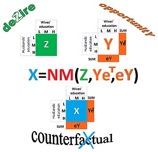
Comparison with the NM-method

Similar to the IPF, the NM-method is also an operation of finding a matrix ${\displaystyle X}$ which is the “closest” to matrix ${\displaystyle Z}$ (${\displaystyle Z\in \mathbb {N} ^{n\times m}}$) while its row totals and column totals are identical to those of a target matrix ${\displaystyle Y}$${\displaystyle (Y\in \mathbb {N} ^{n\times m})}$.

However, there are differences between the NM-method and the IPF. For instance, the NM-method defines closeness of matrices of the same size differently from the IPF. ^[19] Also, the NM-method was developed to solve for matrix ${\displaystyle X}$ in problems, where matrix${\displaystyle {\boldsymbol {Z}}}$is not a sample from the population characterized by the row totals and column totals of matrix ${\displaystyle Y}$, but represents another population. ^[19] In contrast, matrix${\displaystyle {\boldsymbol {Z}}}$is a sample from this population in problems where the IPF is applied as the maximum likelihood estimator .

Macdonald (2023) ^[20] is at ease with the conclusion by Naszodi (2023) ^[21] that the IPF is suitable for sampling correction tasks, but not for generation of counterfactuals. Similarly to Naszodi, Macdonald also questions whether the row and column proportional transformations of the IPF preserve the structure of association within a contingency table that allows us to study social mobility.

Existence and uniqueness of MLEs

Necessary and sufficient conditions for the existence and uniqueness of MLEs are complicated in the general case (see ^[22] ), but sufficient conditions for 2-dimensional tables are simple:

• the marginals of the observed table do not vanish (that is, ${\displaystyle x_{i+}>0,\ x_{+j}>0}$) and
• the observed table is inseparable (i.e. the table does not permute to a block-diagonal shape).

If unique MLEs exist, IPFP exhibits linear convergence in the worst case (Fienberg 1970), but exponential convergence has also been observed (Pukelsheim and Simeone 2009). If a direct estimator (i.e. a closed form of ${\displaystyle ({\hat {m}}_{ij})}$) exists, IPFP converges after 2 iterations. If unique MLEs do not exist, IPFP converges toward the so-called extended MLEs by design (Haberman 1974), but convergence may be arbitrarily slow and often computationally infeasible.

If all observed values are strictly positive, existence and uniqueness of MLEs and therefore convergence is ensured.

Example

Consider the following table, given with the row- and column-sums and targets.

	1	2	3	4	TOTAL	TARGET
1	40	30	20	10	100	150
2	35	50	100	75	260	300
3	30	80	70	120	300	400
4	20	30	40	50	140	150
TOTAL	125	190	230	255	800
TARGET	200	300	400	100		1000

For executing the classical IPFP, we first adjust the rows:

	1	2	3	4	TOTAL	TARGET
1	60.00	45.00	30.00	15.00	150.00	150
2	40.38	57.69	115.38	86.54	300.00	300
3	40.00	106.67	93.33	160.00	400.00	400
4	21.43	32.14	42.86	53.57	150.00	150
TOTAL	161.81	241.50	281.58	315.11	1000.00
TARGET	200	300	400	100		1000

The first step exactly matched row sums, but not the column sums. Next we adjust the columns:

	1	2	3	4	TOTAL	TARGET
1	74.16	55.90	42.62	4.76	177.44	150
2	49.92	71.67	163.91	27.46	312.96	300
3	49.44	132.50	132.59	50.78	365.31	400
4	26.49	39.93	60.88	17.00	144.30	150
TOTAL	200.00	300.00	400.00	100.00	1000.00
TARGET	200	300	400	100		1000

Now the column sums exactly match their targets, but the row sums no longer match theirs. After completing three cycles, each with a row adjustment and a column adjustment, we get a closer approximation:

	1	2	3	4	TOTAL	TARGET
1	64.61	46.28	35.42	3.83	150.13	150
2	49.95	68.15	156.49	25.37	299.96	300
3	56.70	144.40	145.06	53.76	399.92	400
4	28.74	41.18	63.03	17.03	149.99	150
TOTAL	200.00	300.00	400.00	100.00	1000.00
TARGET	200	300	400	100		1000

Implementation

The R package mipfp (currently in version 3.2) provides a multi-dimensional implementation of the traditional iterative proportional fitting procedure. ^[23] The package allows the updating of a N-dimensional array with respect to given target marginal distributions (which, in turn can be multi-dimensional).

Python has an equivalent package, ipfn ^{[24] [25]} that can be installed via pip. The package supports numpy and pandas input objects.

See also

• Data cleansing
• Data editing
• NM-method
• Triangulation (social science) for quantitative and qualitative study data enhancement.

References

1. Bacharach, M. (1965). "Estimating Nonnegative Matrices from Marginal Data". International Economic Review. 6 (3). Blackwell Publishing: 294–310. doi:10.2307/2525582. JSTOR   2525582.
2. Jaynes E.T. (1957) Information theory and statistical mechanics, Physical Review, 106: 620-30.
3. Wilson A.G. (1970) Entropy in urban and regional modelling. London: Pion LTD, Monograph in spatial and environmental systems analysis.
4. Kullback S. & Leibler R.A. (1951) On information and sufficiency, Annals of Mathematics and Statistics, 22 (1951) 79-86.
5. de Mesnard, L. (1994). "Unicity of Biproportion". SIAM Journal on Matrix Analysis and Applications . 15 (2): 490–495. doi:10.1137/S0895479891222507. https://www.researchgate.net/publication/243095013_Unicity_of_Biproportion
6. Kruithof, J (February 1937). "Telefoonverkeersrekening (Calculation of telephone traffic)". De Ingenieur. 52 (8): E15–E25.
7. Deming, W. E.; Stephan, F. F. (1940). "On a Least Squares Adjustment of a Sampled Frequency Table When the Expected Marginal Totals are Known". Annals of Mathematical Statistics . 11 (4): 427–444. doi: 10.1214/aoms/1177731829 . MR   0003527.
8. Lamond, B. and Stewart, N.F. (1981) Bregman's balancing method. Transportation Research 15B, 239-248.
9. Stephan, F. F. (1942). "Iterative method of adjusting frequency tables when expected margins are known". Annals of Mathematical Statistics . 13 (2): 166–178. doi: 10.1214/aoms/1177731604 . MR   0006674. Zbl   0060.31505.
10. Sinkhorn, Richard (1964). “A Relationship Between Arbitrary Positive Matrices and Doubly Stochastic Matrices”. In: Annals of Mathematical Statistics 35.2, pp. 876–879.
11. Bacharach, Michael (1965). “Estimating Nonnegative Matrices from Marginal Data”. In: International Economic Review 6.3, pp. 294–310.
12. Bishop, Y. M. M. (1967). “Multidimensional contingency tables: cell estimates”. PhD thesis. Harvard University.
13. Fienberg, S. E. (1970). "An Iterative Procedure for Estimation in Contingency Tables". Annals of Mathematical Statistics . 41 (3): 907–917. doi: 10.1214/aoms/1177696968 . JSTOR   2239244. MR   0266394. Zbl   0198.23401.
14. Csiszár, I. (1975). "I-Divergence of Probability Distributions and Minimization Problems". Annals of Probability. 3 (1): 146–158. doi: 10.1214/aop/1176996454 . JSTOR   2959270. MR   0365798. Zbl   0318.60013.
15. "On the Iterative Proportional Fitting Procedure: Structure of Accumulation Points and L1-Error Analysis". Pukelsheim, F. and Simeone, B. Retrieved 2009-06-28.
16. Bishop, Y. M. M.; Fienberg, S. E.; Holland, P. W. (1975). Discrete Multivariate Analysis: Theory and Practice. MIT Press. ISBN   978-0-262-02113-5. MR   0381130.
17. Martin Idel (2016) A review of matrix scaling and Sinkhorn’s normal form for matrices and positive maps arXiv preprint https://arxiv.org/pdf/1609.06349.pdf
18. Bradley, A.M. (2010) Algorithms for the equilibration of matrices and their application to limited-memory quasi-newton methods. Ph.D. thesis, Institute for Computational and Mathematical Engineering, Stanford University, 2010
19. Naszodi, A.; Mendonca, F. (2021). "A new method for identifying the role of marital preferences at shaping marriage patterns". Journal of Demographic Economics . 1 (1): 1–27. doi: 10.1017/dem.2021.1 .
20. Macdonald, K. (2023). "The marginal adjustment of mobility tables, revisited". OSF : 1–19.
21. Naszodi, A. (2023). "The iterative proportional fitting algorithm and the NM-method: solutions for two different sets of problems". arXiv: 2303.05515 [econ.GN].
22. Haberman, S. J. (1974). The Analysis of Frequency Data. Univ. Chicago Press. ISBN   978-0-226-31184-5.
23. Barthélemy, Johan; Suesse, Thomas. "mipfp: Multidimensional Iterative Proportional Fitting". CRAN. Retrieved 23 February 2015.
24. "ipfn: pip".
25. "ipfn: github".