
In mathematics, linear interpolation is a method of curve fitting using linear polynomials to construct new data points within the range of a discrete set of known data points.
In mathematics, linear interpolation is a method of curve fitting using linear polynomials to construct new data points within the range of a discrete set of known data points.

If the two known points are given by the coordinates and , the linear interpolant is the straight line between these points. For a value in the interval , the value along the straight line is given from the equation of slopes
which can be derived geometrically from the figure on the right. It is a special case of polynomial interpolation with .
Solving this equation for , which is the unknown value at , gives
which is the formula for linear interpolation in the interval . Outside this interval, the formula is identical to linear extrapolation.
This formula can also be understood as a weighted average. The weights are inversely related to the distance from the end points to the unknown point; the closer point has more influence than the farther point. Thus, the weights are and , which are normalized distances between the unknown point and each of the end points. Because these sum to 1,
yielding the formula for linear interpolation given above.
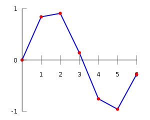
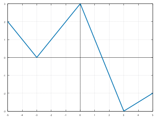
Linear interpolation on a set of data points (x0, y0), (x1, y1), ..., (xn, yn) is defined as piecewise linear, resulting from the concatenation of linear segment interpolants between each pair of data points. This results in a continuous curve, with a discontinuous derivative (in general), thus of differentiability class .
Linear interpolation is often used to approximate a value of some function f using two known values of that function at other points. The error of this approximation is defined as
where p denotes the linear interpolation polynomial defined above:
It can be proven using Rolle's theorem that if f has a continuous second derivative, then the error is bounded by
That is, the approximation between two points on a given function gets worse with the second derivative of the function that is approximated. This is intuitively correct as well: the "curvier" the function is, the worse the approximations made with simple linear interpolation become.
Linear interpolation has been used since antiquity for filling the gaps in tables. Suppose that one has a table listing the population of some country in 1970, 1980, 1990 and 2000, and that one wanted to estimate the population in 1994. Linear interpolation is an easy way to do this. It is believed that it was used in the Seleucid Empire (last three centuries BC) and by the Greek astronomer and mathematician Hipparchus (second century BC). A description of linear interpolation can be found in the ancient Chinese mathematical text called The Nine Chapters on the Mathematical Art (九章算術), [1] dated from 200 BC to AD 100 and the Almagest (2nd century AD) by Ptolemy.
The basic operation of linear interpolation between two values is commonly used in computer graphics. In that field's jargon it is sometimes called a lerp (from linear interpolation). The term can be used as a verb or noun for the operation. e.g. "Bresenham's algorithm lerps incrementally between the two endpoints of the line."
Lerp operations are built into the hardware of all modern computer graphics processors. They are often used as building blocks for more complex operations: for example, a bilinear interpolation can be accomplished in three lerps. Because this operation is cheap, it's also a good way to implement accurate lookup tables with quick lookup for smooth functions without having too many table entries.

If a C0 function is insufficient, for example if the process that has produced the data points is known to be smoother than C0, it is common to replace linear interpolation with spline interpolation or, in some cases, polynomial interpolation.
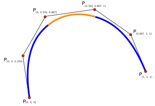
Linear interpolation as described here is for data points in one spatial dimension. For two spatial dimensions, the extension of linear interpolation is called bilinear interpolation, and in three dimensions, trilinear interpolation. Notice, though, that these interpolants are no longer linear functions of the spatial coordinates, rather products of linear functions; this is illustrated by the clearly non-linear example of bilinear interpolation in the figure below. Other extensions of linear interpolation can be applied to other kinds of mesh such as triangular and tetrahedral meshes, including Bézier surfaces. These may be defined as indeed higher-dimensional piecewise linear functions (see second figure below).


Many libraries and shading languages have a "lerp" helper-function (in GLSL known instead as mix), returning an interpolation between two inputs (v0, v1) for a parameter t in the closed unit interval [0, 1]. Signatures between lerp functions are variously implemented in both the forms (v0, v1, t) and (t, v0, v1).
// Imprecise method, which does not guarantee v = v1 when t = 1, due to floating-point arithmetic error.// This method is monotonic. This form may be used when the hardware has a native fused multiply-add instruction.floatlerp(floatv0,floatv1,floatt){returnv0+t*(v1-v0);}// Precise method, which guarantees v = v1 when t = 1. This method is monotonic only when v0 * v1 < 0.// Lerping between same values might not produce the same valuefloatlerp(floatv0,floatv1,floatt){return(1-t)*v0+t*v1;}This lerp function is commonly used for alpha blending (the parameter "t" is the "alpha value"), and the formula may be extended to blend multiple components of a vector (such as spatial x, y, z axes or r, g, b colour components) in parallel.
In mathematics, an equation is a mathematical formula that expresses the equality of two expressions, by connecting them with the equals sign =. The word equation and its cognates in other languages may have subtly different meanings; for example, in French an équation is defined as containing one or more variables, while in English, any well-formed formula consisting of two expressions related with an equals sign is an equation.

In the mathematical field of numerical analysis, interpolation is a type of estimation, a method of constructing (finding) new data points based on the range of a discrete set of known data points.
A finite difference is a mathematical expression of the form f (x + b) − f (x + a). If a finite difference is divided by b − a, one gets a difference quotient. The approximation of derivatives by finite differences plays a central role in finite difference methods for the numerical solution of differential equations, especially boundary value problems.

In analysis, numerical integration comprises a broad family of algorithms for calculating the numerical value of a definite integral. The term numerical quadrature is more or less a synonym for "numerical integration", especially as applied to one-dimensional integrals. Some authors refer to numerical integration over more than one dimension as cubature; others take "quadrature" to include higher-dimensional integration.

The Chebyshev polynomials are two sequences of polynomials related to the cosine and sine functions, notated as and . They can be defined in several equivalent ways, one of which starts with trigonometric functions:

In the mathematical field of numerical analysis, Runge's phenomenon is a problem of oscillation at the edges of an interval that occurs when using polynomial interpolation with polynomials of high degree over a set of equispaced interpolation points. It was discovered by Carl David Tolmé Runge (1901) when exploring the behavior of errors when using polynomial interpolation to approximate certain functions. The discovery shows that going to higher degrees does not always improve accuracy. The phenomenon is similar to the Gibbs phenomenon in Fourier series approximations.
In numerical analysis, polynomial interpolation is the interpolation of a given bivariate data set by the polynomial of lowest possible degree that passes through the points of the dataset.
In the mathematical field of numerical analysis, a Newton polynomial, named after its inventor Isaac Newton, is an interpolation polynomial for a given set of data points. The Newton polynomial is sometimes called Newton's divided differences interpolation polynomial because the coefficients of the polynomial are calculated using Newton's divided differences method.

In numerical analysis, the Lagrange interpolating polynomial is the unique polynomial of lowest degree that interpolates a given set of data.
In mathematics, a piecewise-defined function is a function whose domain is partitioned into several intervals ("subdomains") on which the function may be defined differently. Piecewise definition is actually a way of specifying the function, rather than a characteristic of the resulting function itself.
In mathematics, a spline is a function defined piecewise by polynomials. In interpolating problems, spline interpolation is often preferred to polynomial interpolation because it yields similar results, even when using low degree polynomials, while avoiding Runge's phenomenon for higher degrees.

In mathematics, extrapolation is a type of estimation, beyond the original observation range, of the value of a variable on the basis of its relationship with another variable. It is similar to interpolation, which produces estimates between known observations, but extrapolation is subject to greater uncertainty and a higher risk of producing meaningless results. Extrapolation may also mean extension of a method, assuming similar methods will be applicable. Extrapolation may also apply to human experience to project, extend, or expand known experience into an area not known or previously experienced so as to arrive at a knowledge of the unknown. The extrapolation method can be applied in the interior reconstruction problem.
In the mathematical field of numerical analysis, spline interpolation is a form of interpolation where the interpolant is a special type of piecewise polynomial called a spline. That is, instead of fitting a single, high-degree polynomial to all of the values at once, spline interpolation fits low-degree polynomials to small subsets of the values, for example, fitting nine cubic polynomials between each of the pairs of ten points, instead of fitting a single degree-nine polynomial to all of them. Spline interpolation is often preferred over polynomial interpolation because the interpolation error can be made small even when using low-degree polynomials for the spline. Spline interpolation also avoids the problem of Runge's phenomenon, in which oscillation can occur between points when interpolating using high-degree polynomials.

In mathematics, bilinear interpolation is a method for interpolating functions of two variables using repeated linear interpolation. It is usually applied to functions sampled on a 2D rectilinear grid, though it can be generalized to functions defined on the vertices of arbitrary convex quadrilaterals.
In mathematics, trigonometric interpolation is interpolation with trigonometric polynomials. Interpolation is the process of finding a function which goes through some given data points. For trigonometric interpolation, this function has to be a trigonometric polynomial, that is, a sum of sines and cosines of given periods. This form is especially suited for interpolation of periodic functions.
In mathematics, the Lebesgue constants (depending on a set of nodes and of its size) give an idea of how good the interpolant of a function (at the given nodes) is in comparison with the best polynomial approximation of the function (the degree of the polynomials are fixed). The Lebesgue constant for polynomials of degree at most n and for the set of n + 1 nodes T is generally denoted by Λn(T ). These constants are named after Henri Lebesgue.
In numerical analysis, Hermite interpolation, named after Charles Hermite, is a method of polynomial interpolation, which generalizes Lagrange interpolation. Lagrange interpolation allows computing a polynomial of degree less than n that takes the same value at n given points as a given function. Instead, Hermite interpolation computes a polynomial of degree less than mn such that the polynomial and its first m − 1 derivatives have the same values at n given points as a given function and its first m − 1 derivatives.
In numerical analysis, multivariate interpolation is interpolation on functions of more than one variable ; when the variates are spatial coordinates, it is also known as spatial interpolation.
In algebra, a multilinear polynomial is a multivariate polynomial that is linear in each of its variables separately, but not necessarily simultaneously. It is a polynomial in which no variable occurs to a power of 2 or higher; that is, each monomial is a constant times a product of distinct variables. For example f(x,y,z) = 3xy + 2.5 y - 7z is a multilinear polynomial of degree 2 whereas f(x,y,z) = x² +4y is not. The degree of a multilinear polynomial is the maximum number of distinct variables occurring in any monomial.


