There are two prevailing definitions, denoted here as rounding machine epsilon and interval machine epsilon. The machine epsilon is dependent on the type of rounding used and is also called unit roundoff, which has the symbol bold Roman u. However, in the commonly used definition, machine epsilon is independent of rounding method, and may be equivalent to u or 2u.
Values for standard hardware arithmetics
The following table lists machine epsilon values for standard floating-point formats.
↑ According to formal definition — used by Prof. Demmel, LAPACK and Scilab. It represents the largest relative rounding error in round-to-nearest mode. The rationale is that the rounding error is half the interval upwards to the next representable number in finite-precision. Thus, the relative rounding error for number is . In this context, the largest relative error occurs when , and is equal to , because real numbers in the lower half of the interval 1.0 ~ 1.0+ULP(1) are rounded down to 1.0, and numbers in the upper half of the interval are rounded up to 1.0+ULP(1). Here we use the definition of ULP(1) (Unit in Last Place) as the positive difference between 1.0 (which can be represented exactly in finite-precision) and the next greater number representable in finite-precision.
↑ According to the mainstream definition — used by Prof. Higham; applied in language constants in Ada, C, C++, Fortran, MATLAB, Mathematica, Octave, Pascal, Python and Rust etc., and defined in textbooks like «Numerical Recipes» by Press et al. It represents the largest relative interval between two nearest numbers in finite-precision, or the largest rounding error in round-by-chop mode. The rationale is that the relative interval for number is where is the distance to upwards the next representable number in finite-precision. In this context, the largest relative interval occurs when , and is the interval between 1.0 (which can be represented exactly in finite-precision) and the next larger representable floating-point number. This interval is equal to ULP(1).
Formal definition (Rounding machine epsilon)
Rounding is a procedure for choosing the representation of a real number in a floating point number system. For a number system and a rounding procedure, machine epsilon is the maximum relative error of the chosen rounding procedure.
Some background is needed to determine a value from this definition. A floating point number system is characterized by a radix which is also called the base, , and by the precision, i.e. the number of radix digits of the significand (including any leading implicit bit). All the numbers with the same exponent, , have the spacing, . The spacing changes at the numbers that are perfect powers of ; the spacing on the side of larger magnitude is times larger than the spacing on the side of smaller magnitude.
Since machine epsilon is a bound for relative error, it suffices to consider numbers with exponent . It also suffices to consider positive numbers. For the usual round-to-nearest kind of rounding, the absolute rounding error is at most half the spacing, or . This value is the biggest possible numerator for the relative error. The denominator in the relative error is the number being rounded, which should be as small as possible to make the relative error large. The worst relative error therefore happens when rounding is applied to numbers of the form where is between and . All these numbers round to with relative error . The maximum occurs when is at the upper end of its range. The in the denominator is negligible compared to the numerator, so it is left off for expediency, and just is taken as machine epsilon. As has been shown here, the relative error is worst for numbers that round to , so machine epsilon also is called unit roundoff meaning roughly "the maximum error that can occur when rounding to the unit value".
Thus, the maximum spacing between a normalised floating point number, , and an adjacent normalised number is .[3]
Arithmetic model
Numerical analysis uses machine epsilon to study the effects of rounding error. The actual errors of machine arithmetic are far too complicated to be studied directly, so instead, the following simple model is used. The IEEE arithmetic standard says all floating-point operations are done as if it were possible to perform the infinite-precision operation, and then, the result is rounded to a floating-point number. Suppose (1) , are floating-point numbers, (2) is an arithmetic operation on floating-point numbers such as addition or multiplication, and (3) is the infinite precision operation. According to the standard, the computer calculates:
By the meaning of machine epsilon, the relative error of the rounding is at most machine epsilon in magnitude, so:
where in absolute magnitude is at most or u. The books by Demmel and Higham in the references can be consulted to see how this model is used to analyze the errors of, say, Gaussian elimination.
Mainstream definition (Interval machine epsilon)
The IEEE standard does not define the terms machine epsilon and unit roundoff, so differing definitions of these terms are in use, which can cause some confusion.
The formal definition for machine epsilon is the one used by Prof. James Demmel in lecture scripts,[4] the LAPACK linear algebra package,[5] numerics research papers[6] and some scientific computing software.[7] Most numerical analysts use the words machine epsilon and unit roundoff interchangeably with this meaning.
This alternative definition is significantly more widespread: machine epsilon is the difference between 1 and the next larger floating point number.
By this definition, ε equals the value of the unit in the last place relative to 1, i.e. (where b is the base of the floating point system and p is the precision) and the unit roundoff is u = ε / 2, assuming round-to-nearest mode, and u = ε, assuming round-by-chop.
The prevalence of this definition is rooted in its use in the ISO C Standard for constants relating to floating-point types[8][9] and corresponding constants in other programming languages.[10][11][12] It is also widely used in scientific computing software[13][14][15] and in the numerics and computing literature.[16][17][18][19]
How to determine machine epsilon
Where standard libraries do not provide precomputed values (as <float.h> does with FLT_EPSILON, DBL_EPSILON and LDBL_EPSILON for C and <limits> does with std::numeric_limits<T>::epsilon() in C++), the best way to determine machine epsilon is to refer to the table, above, and use the appropriate power formula. Computing machine epsilon is often given as a textbook exercise. The following examples compute interval machine epsilon in the sense of the spacing of the floating point numbers at 1 rather than in the sense of the unit roundoff.
Note that results depend on the particular floating-point format used, such as float, double, long double, or similar as supported by the programming language, the compiler, and the runtime library for the actual platform.
Some formats supported by the processor might not be supported by the chosen compiler and operating system. Other formats might be emulated by the runtime library, including arbitrary-precision arithmetic available in some languages and libraries.
In a strict sense the term machine epsilon means the accuracy directly supported by the processor (or coprocessor), not some accuracy supported by a specific compiler for a specific operating system, unless it's known to use the best format.
IEEE 754 floating-point formats have the property that, when reinterpreted as a two's complement integer of the same width, they monotonically increase over positive values and monotonically decrease over negative values (see the binary representation of 32 bit floats). They also have the property that , and (where is the aforementioned integer reinterpretation of ). In languages that allow type punning and always use IEEE 754–1985, we can exploit this to compute a machine epsilon in constant time. For example, in C:
The machine epsilon, can also simply be calculated as two to the negative power of the number of bits used for the mantissa.
Relationship to absolute relative error
If is the machine representation of a number then the absolute relative error in the representation is [20]
Proof
The following proof is limited to positive numbers and machine representations using round-by-chop.
If is a positive number we want to represent, it will be between a machine number below and a machine number above .
If , where is the number of bits used for the magnitude of the significand, then:
Since the representation of will be either or ,
Although this proof is limited to positive numbers and round-by-chop, the same method can be used to prove the inequality in relation to negative numbers and round-to-nearest machine representations.
See also
Floating point, general discussion of accuracy issues in floating point arithmetic
↑ Extended Pascal ISO 10206:1990 (Technical report). The value of epsreal shall be the result of subtracting 1.0 from the smallest value of real-type that is greater than 1.0.
Anderson, E.; LAPACK Users' Guide, Society for Industrial and Applied Mathematics (SIAM), Philadelphia, PA, third edition, 1999.
Cody, William J.; MACHAR: A Soubroutine to Dynamically Determine Machine Parameters, ACM Transactions on Mathematical Software, Vol. 14(4), 1988, 303–311.
Besset, Didier H.; Object-Oriented Implementation of Numerical Methods, Morgan & Kaufmann, San Francisco, CA, 2000.
Demmel, James W., Applied Numerical Linear Algebra, Society for Industrial and Applied Mathematics (SIAM), Philadelphia, PA, 1997.
Higham, Nicholas J.; Accuracy and Stability of Numerical Algorithms, Society for Industrial and Applied Mathematics (SIAM), Philadelphia, PA, second edition, 2002.
Press, William H.; Teukolsky, Saul A.; Vetterling, William T.; and Flannery, Brian P.; Numerical Recipes in Fortran 77, 2nd ed., Chap. 20.2, pp.881–886
Forsythe, George E.; Malcolm, Michael A.; Moler, Cleve B.; "Computer Methods for Mathematical Computations", Prentice-Hall, ISBN0-13-165332-6, 1977
External links
MACHAR, a routine (in C and Fortran) to "dynamically compute machine constants" (ACM algorithm 722)
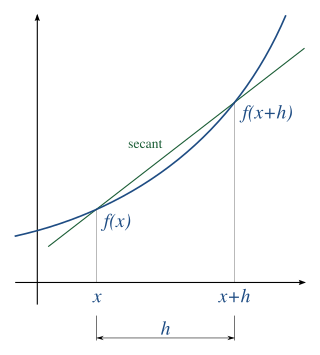
In numerical analysis, the condition number of a function measures how much the output value of the function can change for a small change in the input argument. This is used to measure how sensitive a function is to changes or errors in the input, and how much error in the output results from an error in the input. Very frequently, one is solving the inverse problem: given one is solving for x, and thus the condition number of the (local) inverse must be used.
In computing, floating-point arithmetic (FP) is arithmetic that represents subsets of real numbers using an integer with a fixed precision, called the significand, scaled by an integer exponent of a fixed base. Numbers of this form are called floating-point numbers. For example, 12.345 is a floating-point number in base ten with five digits of precision:
In mathematics, the branch of real analysis studies the behavior of real numbers, sequences and series of real numbers, and real functions. Some particular properties of real-valued sequences and functions that real analysis studies include convergence, limits, continuity, smoothness, differentiability and integrability.
In numerical analysis, a root-finding algorithm is an algorithm for finding zeros, also called "roots", of continuous functions. A zero of a function f, from the real numbers to real numbers or from the complex numbers to the complex numbers, is a number x such that f(x) = 0. As, generally, the zeros of a function cannot be computed exactly nor expressed in closed form, root-finding algorithms provide approximations to zeros, expressed either as floating-point numbers or as small isolating intervals, or disks for complex roots (an interval or disk output being equivalent to an approximate output together with an error bound).
In mathematics, the limit of a function is a fundamental concept in calculus and analysis concerning the behavior of that function near a particular input which may or may not be in the domain of the function.
In mathematics, the limit of a sequence is the value that the terms of a sequence "tend to", and is often denoted using the symbol. If such a limit exists, the sequence is called convergent. A sequence that does not converge is said to be divergent. The limit of a sequence is said to be the fundamental notion on which the whole of mathematical analysis ultimately rests.
In numerical analysis, the Kahan summation algorithm, also known as compensated summation, significantly reduces the numerical error in the total obtained by adding a sequence of finite-precision floating-point numbers, compared to the obvious approach. This is done by keeping a separate running compensation, in effect extending the precision of the sum by the precision of the compensation variable.
In computing, a roundoff error, also called rounding error, is the difference between the result produced by a given algorithm using exact arithmetic and the result produced by the same algorithm using finite-precision, rounded arithmetic. Rounding errors are due to inexactness in the representation of real numbers and the arithmetic operations done with them. This is a form of quantization error. When using approximation equations or algorithms, especially when using finitely many digits to represent real numbers, one of the goals of numerical analysis is to estimate computation errors. Computation errors, also called numerical errors, include both truncation errors and roundoff errors.
The approximation error in a data value is the discrepancy between an exact value and some approximation to it. This error can be expressed as an absolute error or as a relative error.
In mathematics, nonstandard calculus is the modern application of infinitesimals, in the sense of nonstandard analysis, to infinitesimal calculus. It provides a rigorous justification for some arguments in calculus that were previously considered merely heuristic.
In mathematics, the bisection method is a root-finding method that applies to any continuous function for which one knows two values with opposite signs. The method consists of repeatedly bisecting the interval defined by these values and then selecting the subinterval in which the function changes sign, and therefore must contain a root. It is a very simple and robust method, but it is also relatively slow. Because of this, it is often used to obtain a rough approximation to a solution which is then used as a starting point for more rapidly converging methods. The method is also called the interval halving method, the binary search method, or the dichotomy method.
In mathematics and computer algebra, automatic differentiation, also called algorithmic differentiation, computational differentiation, is a set of techniques to evaluate the partial derivative of a function specified by a computer program.
In mathematics, approximation theory is concerned with how functions can best be approximated with simpler functions, and with quantitatively characterizing the errors introduced thereby. What is meant by best and simpler will depend on the application.
In numerical analysis, numerical differentiation algorithms estimate the derivative of a mathematical function or function subroutine using values of the function and perhaps other knowledge about the function.
Interval arithmetic is a mathematical technique used to mitigate rounding and measurement errors in mathematical computation by computing function bounds. Numerical methods involving interval arithmetic can guarantee relatively reliable and mathematically correct results. Instead of representing a value as a single number, interval arithmetic or interval mathematics represents each value as a range of possibilities.
Affine arithmetic (AA) is a model for self-validated numerical analysis. In AA, the quantities of interest are represented as affine combinations of certain primitive variables, which stand for sources of uncertainty in the data or approximations made during the computation.
Methods of computing square roots are algorithms for approximating the non-negative square root of a positive real number . Since all square roots of natural numbers, other than of perfect squares, are irrational, square roots can usually only be computed to some finite precision: these methods typically construct a series of increasingly accurate approximations.
Adaptive Simpson's method, also called adaptive Simpson's rule, is a method of numerical integration proposed by G.F. Kuncir in 1962. It is probably the first recursive adaptive algorithm for numerical integration to appear in print, although more modern adaptive methods based on Gauss–Kronrod quadrature and Clenshaw–Curtis quadrature are now generally preferred. Adaptive Simpson's method uses an estimate of the error we get from calculating a definite integral using Simpson's rule. If the error exceeds a user-specified tolerance, the algorithm calls for subdividing the interval of integration in two and applying adaptive Simpson's method to each subinterval in a recursive manner. The technique is usually much more efficient than composite Simpson's rule since it uses fewer function evaluations in places where the function is well-approximated by a cubic function.
In numerical analysis, catastrophic cancellation is the phenomenon that subtracting good approximations to two nearby numbers may yield a very bad approximation to the difference of the original numbers.
In numerical analysis, pairwise summation, also called cascade summation, is a technique to sum a sequence of finite-precision floating-point numbers that substantially reduces the accumulated round-off error compared to naively accumulating the sum in sequence. Although there are other techniques such as Kahan summation that typically have even smaller round-off errors, pairwise summation is nearly as good while having much lower computational cost—it can be implemented so as to have nearly the same cost as naive summation.
This page is based on this Wikipedia article Text is available under the CC BY-SA 4.0 license; additional terms may apply. Images, videos and audio are available under their respective licenses.