Multitrait-multimethod matrix

Last updated

The multitrait-multimethod (MTMM) matrix is an approach to examining construct validity developed by Campbell and Fiske (1959). [1] It organizes convergent and discriminant validity evidence for comparison of how a measure relates to other measures. The conceptual approach has influenced experimental design and measurement theory in psychology, including applications in structural equation models.

Contents

Definitions and key components

Multiple traits are used in this approach to examine (a) similar or (b) dissimilar traits (constructs), in order to establish convergent and discriminant validity between traits. Similarly, multiple methods are used in this approach to examine the differential effects (or lack thereof) caused by method specific variance. Scores could be correlated because they measure similar traits, or because they are based on similar methods, or both. When variables that are supposed to measure different constructs show a high correlation because they based on similar methods, this is sometimes described as a "nuisance variance" or "method bias" problem. [2]

There are six major considerations when examining a construct's validity through the MTMM matrix, which are as follows:

  1. Evaluation of convergent validity Tests designed to measure the same construct should correlate highly amongst themselves.
  2. Evaluation of discriminant (divergent) validity The construct being measured by a test should not correlate highly with different constructs.
  3. Trait-method unit- Each task or test used in measuring a construct is considered a trait-method unit; in that the variance contained in the measure is part trait, and part method. Generally, researchers desire low method-specific variance and high trait variance.
  4. Multitrait-multimethod More than one trait and more than one method must be used to establish (a) discriminant validity and (b) the relative contributions of the trait or method-specific variance. This tenet is consistent with the ideas proposed in Platt's concept of Strong inference (1964). [3]
  5. Truly different methodology When using multiple methods, one must consider how different the actual measures are. For instance, delivering two self-report measures are not truly different measures; whereas using an interview scale or a psychosomatic reading would be.
  6. Trait characteristics Traits should be different enough to be distinct, but similar enough to be worth examining in the MTMM.

Example

The example below provides a prototypical matrix and what the correlations between measures mean. The diagonal line is typically filled in with a reliability coefficient of the measure (e.g. alpha coefficient). Descriptions in brackets [] indicate what is expected when the validity of the construct (e.g., depression or anxiety) and the validities of the measures are all high.

Test Beck Depression Inventory (BDI) - Questionnaire Hamilton Depression Rating Scale (HDRS) - Interview Beck Anxiety Inventory (BAI) - QuestionnaireClinician Global Impressions - Anxiety (CGI-A) - Interview
BDI(Reliability Coefficient)

[close to 1.00]

HDRSHeteromethod-monotrait

[highest of all except reliability]

(Reliability Coefficient)

[close to 1.00]

BAIMonomethod-heterotrait

[low, less than monotrait]

Heteromethod-heterotrait

[lowest of all]

(Reliability Coefficient) [close to 1.00]
CGI-AHeteromethod-heterotrait

[lowest of all]

Monomethod-heterotrait

[low, less than monotrait]

Heteromethod-monotrait

[highest of all except reliability]

(Reliability Coefficient)

[close to 1.00]

In this example, the first row lists the trait being assessed (i.e., depression or anxiety) as well as the method of assessing this trait (i.e., self-reported questionnaire versus an interview). The term heteromethod indicates this cell reports the correlation between two separate methods. Monomethod indicates that the same method is being used instead (e.g., interview and interview). Heterotrait indicates that the cell refers to two supposedly different traits. Monotrait indicates the same trait supposed to be measured.

This framework makes it clear that there are at least two sources of variance that can influence observed scores on a measure: Not just the underlying trait (which is usually the goal of gathering the measurement in the first place), but also the method used to gather the measurement. The MTMM matrix uses two or more measures of each trait and two or more methods to start to tease apart the contributions of different factors. The first frame of the animated figure shows how the four measurements in the table are paired in terms of focusing on the "traits" of depression (BDI and HDRS) and anxiety (BAI and CGI-A). The second shows that they are also paired in terms of source method: two use self-report questionnaires (often referred to as "surveys"), and two are based on interview (which can incorporate direct observation of nonverbal communication and behavior, as well as the interviewee's response).

Scores on each measure are influenced by both the trait and also the method by which the information is gathered Multi-Trait, Multi-Method (MTMM) example.gif
Scores on each measure are influenced by both the trait and also the method by which the information is gathered

With observed data, it is possible to examine the proportion of variance shared among traits and methods to gain a sense of how much method-specific variance is induced by the measurement method, as well as provide a look at how distinct the trait is, as compared to another trait.

Ideally, the trait should matter more than the specific method chosen for measurement. For example, if a person is measured as being highly depressed by one measure, then another depression measure should also yield high scores. On the other hand, people who appear highly depressed on the Beck Depression Inventory should not necessarily get high anxiety scores on Beck's Anxiety Inventory, inasmuch as they are supposed to be measuring different constructs. Since the inventories were written by the same person, and are similar in style, there might be some correlation, but this similarity in method should not affect the scores much, so the correlations between these measures of different traits should be low.

Analysis

A variety of statistical approaches have been used to analyze the data from the MTMM matrix. The standard method from Campbell and Fiske can be implemented using the MTMM.EXE program available at: https://web.archive.org/web/20160304173400/http://gim.med.ucla.edu/FacultyPages/Hays/utils/ One can also use confirmatory factor analysis [4] due to the complexities in considering all of the data in the matrix. The Sawilowsky I test, [5] [6] however, considers all of the data in the matrix with a distribution-free statistical test for trend.

Example of a MTMM measurement model MTMM model.PNG
Example of a MTMM measurement model

The test is conducted by reducing the heterotrait-heteromethod and heterotrait-monomethod triangles, and the validity and reliability diagonals, into a matrix of four levels. Each level consists of the minimum, median, and maximum value. The null hypothesis is these values are unordered, which is tested against the alternative hypothesis of an increasing ordered trend. The test statistic is found by counting the number of inversions (I). The critical value for alpha = 0.05 is 10, and for alpha = .01 is 14.


One of the most used models to analyze MTMM data is the True Score model proposed by Saris and Andrews ( [7] ). The True Score model can be expressed using the following standardized equations:

    1) Yij = rijTSij + eij* where:          Yij is the standardized observed variable measured with the ith trait and jth method.          rij is the reliability coefficient, which is equal to:            rij = σYij / σTSijTSij is the standardized true score variable          eij* is the random error, which is equal to:            eij* = eij / σYij             Consequently:        rij2 = 1 - σ2(eij*) where:          rij2 is the reliability
    2) TSij = vijFi + mijMj where:          vij is the validity coefficient, which is equal to:            vij = σFi / σTSijFi is the standardized latent factor for the ith variable of interest (or trait)          mij is the method effect, which is equal to:          mij = σMj / σTSijMj is the standardized latent factor for the reaction to the jthmethod             Consequently:        vij2 = 1 - mij2 where:          vij2 is the validity
    3) Yij = qijFi + rijmijMj + e* where:          qij is the quality coefficient, which is equal to:            qij = rij vij               Consequently:        qij2 = rij2 vij2 = σ2Fi / σ2Yij where:          qij2 is the quality

The assumptions are the following:

     * The errors are random, thus the mean of the errors is zero: µe = E(e) = 0       * The random errors are uncorrelated with each other: cov(ei, ej) = E(ei ej) = 0       * The random errors are uncorrelated with the independent variables:  cov(TS, e) = E(TS e) = 0 ,  cov(F, e) = E(F e) = 0  and  cov(M, e) = E(M e) = 0        * The method factors are assumed to be uncorrelated with one another and with the trait factors: cov(F, M) = E(F M) = 0 


Typically, the respondent must answer at least three different measures (i.e., traits) measured using at least three different methods. This model has been used to estimate the quality of thousands of survey questions, in particular in the frame of the European Social Survey.


Related Research Articles

<span class="mw-page-title-main">Variance</span> Statistical measure of how far values spread from their average

In probability theory and statistics, variance is the expectation of the squared deviation of a random variable from its population mean or sample mean. Variance is a measure of dispersion, meaning it is a measure of how far a set of numbers is spread out from their average value. Variance has a central role in statistics, where some ideas that use it include descriptive statistics, statistical inference, hypothesis testing, goodness of fit, and Monte Carlo sampling. Variance is an important tool in the sciences, where statistical analysis of data is common. The variance is the square of the standard deviation, the second central moment of a distribution, and the covariance of the random variable with itself, and it is often represented by , , , , or .

<span class="mw-page-title-main">Correlation</span> Statistical concept

In statistics, correlation or dependence is any statistical relationship, whether causal or not, between two random variables or bivariate data. Although in the broadest sense, "correlation" may indicate any type of association, in statistics it normally refers to the degree to which a pair of variables are linearly related. Familiar examples of dependent phenomena include the correlation between the height of parents and their offspring, and the correlation between the price of a good and the quantity the consumers are willing to purchase, as it is depicted in the so-called demand curve.

<span class="mw-page-title-main">Pearson correlation coefficient</span> Measure of linear correlation

In statistics, the Pearson correlation coefficient ― also known as Pearson's r, the Pearson product-moment correlation coefficient (PPMCC), the bivariate correlation, or colloquially simply as the correlation coefficient ― is a measure of linear correlation between two sets of data. It is the ratio between the covariance of two variables and the product of their standard deviations; thus, it is essentially a normalized measurement of the covariance, such that the result always has a value between −1 and 1. As with covariance itself, the measure can only reflect a linear correlation of variables, and ignores many other types of relationships or correlations. As a simple example, one would expect the age and height of a sample of teenagers from a high school to have a Pearson correlation coefficient significantly greater than 0, but less than 1.

<span class="mw-page-title-main">Spearman's rank correlation coefficient</span> Nonparametric measure of rank correlation

In statistics, Spearman's rank correlation coefficient or Spearman's ρ, named after Charles Spearman and often denoted by the Greek letter (rho) or as , is a nonparametric measure of rank correlation. It assesses how well the relationship between two variables can be described using a monotonic function.

In statistics and psychometrics, reliability is the overall consistency of a measure. A measure is said to have a high reliability if it produces similar results under consistent conditions:

"It is the characteristic of a set of test scores that relates to the amount of random error from the measurement process that might be embedded in the scores. Scores that are highly reliable are precise, reproducible, and consistent from one testing occasion to another. That is, if the testing process were repeated with a group of test takers, essentially the same results would be obtained. Various kinds of reliability coefficients, with values ranging between 0.00 and 1.00, are usually used to indicate the amount of error in the scores."

In the social sciences, scaling is the process of measuring or ordering entities with respect to quantitative attributes or traits. For example, a scaling technique might involve estimating individuals' levels of extraversion, or the perceived quality of products. Certain methods of scaling permit estimation of magnitudes on a continuum, while other methods provide only for relative ordering of the entities.

Canonical correlation Way of inferring information from cross-covariance matrices

In statistics, canonical-correlation analysis (CCA), also called canonical variates analysis, is a way of inferring information from cross-covariance matrices. If we have two vectors X = (X1, ..., Xn) and Y = (Y1, ..., Ym) of random variables, and there are correlations among the variables, then canonical-correlation analysis will find linear combinations of X and Y which have maximum correlation with each other. T. R. Knapp notes that "virtually all of the commonly encountered parametric tests of significance can be treated as special cases of canonical-correlation analysis, which is the general procedure for investigating the relationships between two sets of variables." The method was first introduced by Harold Hotelling in 1936, although in the context of angles between flats the mathematical concept was published by Jordan in 1875.

Cronbach's alpha, also known as tau-equivalent reliability or coefficient alpha, is a reliability coefficient that provides a method of measuring internal consistency of tests.

Construct validity is the accumulation of evidence to support the interpretation of what a measure reflects. Modern validity theory defines construct validity as the overarching concern of validity research, subsuming all other types of validity evidence such as content validity and criterion validity.

Linear discriminant analysis (LDA), normal discriminant analysis (NDA), or discriminant function analysis is a generalization of Fisher's linear discriminant, a method used in statistics and other fields, to find a linear combination of features that characterizes or separates two or more classes of objects or events. The resulting combination may be used as a linear classifier, or, more commonly, for dimensionality reduction before later classification.

Personality Assessment Inventory (PAI), developed by Leslie Morey, is a self-report 344-item personality test that assesses a respondent's personality and psychopathology. Each item is a statement about the respondent that the respondent rates with a 4-point scale. It is used in various contexts, including psychotherapy, crisis/evaluation, forensic, personnel selection, pain/medical, and child custody assessment. The test construction strategy for the PAI was primarily deductive and rational. It shows good convergent validity with other personality tests, such as the Minnesota Multiphasic Personality Inventory and the Revised NEO Personality Inventory.

Convergent validity, for human cognition, especially within sociology, psychology, and other behavioral sciences, refers to the degree to which two measures that theoretically should be related, are in fact related. Convergent validity, along with discriminant validity, is a subtype of construct validity. Convergent validity can be established if two similar constructs correspond with one another, while discriminant validity applies to two dissimilar constructs that are easily differentiated.

In psychology, discriminant validity tests whether concepts or measurements that are not supposed to be related are actually unrelated.

In probability theory and statistics, partial correlation measures the degree of association between two random variables, with the effect of a set of controlling random variables removed. If we are interested in finding to what extent there is a numerical relationship between two variables of interest, using their correlation coefficient will give misleading results if there is another, confounding, variable that is numerically related to both variables of interest. This misleading information can be avoided by controlling for the confounding variable, which is done by computing the partial correlation coefficient. This is precisely the motivation for including other right-side variables in a multiple regression; but while multiple regression gives unbiased results for the effect size, it does not give a numerical value of a measure of the strength of the relationship between the two variables of interest.

In statistics, confirmatory factor analysis (CFA) is a special form of factor analysis, most commonly used in social research. It is used to test whether measures of a construct are consistent with a researcher's understanding of the nature of that construct. As such, the objective of confirmatory factor analysis is to test whether the data fit a hypothesized measurement model. This hypothesized model is based on theory and/or previous analytic research. CFA was first developed by Jöreskog (1969) and has built upon and replaced older methods of analyzing construct validity such as the MTMM Matrix as described in Campbell & Fiske (1959).

Intraclass correlation Descriptive statistic

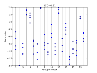
In statistics, the intraclass correlation, or the intraclass correlation coefficient (ICC), is a descriptive statistic that can be used when quantitative measurements are made on units that are organized into groups. It describes how strongly units in the same group resemble each other. While it is viewed as a type of correlation, unlike most other correlation measures it operates on data structured as groups, rather than data structured as paired observations.

Multivariate analysis of covariance (MANCOVA) is an extension of analysis of covariance (ANCOVA) methods to cover cases where there is more than one dependent variable and where the control of concomitant continuous independent variables – covariates – is required. The most prominent benefit of the MANCOVA design over the simple MANOVA is the 'factoring out' of noise or error that has been introduced by the covariant. A commonly used multivariate version of the ANOVA F-statistic is Wilks' Lambda (Λ), which represents the ratio between the error variance and the effect variance.

The person–situation debate in personality psychology refers to the controversy concerning whether the person or the situation is more influential in determining a person's behavior. Personality trait psychologists believe that a person's personality is relatively consistent across situations. Situationists, opponents of the trait approach, argue that people are not consistent enough from situation to situation to be characterized by broad personality traits. The debate is also an important discussion when studying social psychology, as both topics address the various ways a person could react to a given situation.

<span class="mw-page-title-main">Average variance extracted</span>

In statistics, average variance extracted (AVE) is a measure of the amount of variance that is captured by a construct in relation to the amount of variance due to measurement error.

<span class="mw-page-title-main">Homoscedasticity and heteroscedasticity</span> Statistical property

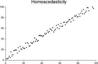
In statistics, a sequence of random variables is homoscedastic if all its random variables have the same finite variance. This is also known as homogeneity of variance. The complementary notion is called heteroscedasticity. The spellings homoskedasticity and heteroskedasticity are also frequently used.

References

  1. Campbell, D.T., & FiskeD.W. (1959) Convergent and discriminant validation by the multitrait-multimethod matrix. Psychological Bulletin, 56, 81-105 "
  2. Podsakoff, Philip M.; MacKenzie, Scott B.; Podsakoff, Nathan P. (2012-01-10). "Sources of Method Bias in Social Science Research and Recommendations on How to Control It". Annual Review of Psychology. 63 (1): 539–569. doi:10.1146/annurev-psych-120710-100452. ISSN   0066-4308.
  3. John R. Platt (1964). "Strong inference". Science 146 (3642). 
  4. Figueredo, A., Ferketich, S., Knapp, T. (1991). Focus on psychometrics: More on MTMM: The Role of Confirmatory Factor Analysis. Nursing & Health, 14, 387-391
  5. Sawilowsky, S. (2002). A quick distribution-free test for trend that contributes evidence of construct validity. Measurement and Evaluation in Counseling and Development, 35, 78-88.
  6. Cuzzocrea, J., & Sawilowsky, S. (2009). Robustness to non-independence and power of the I test for trend in construct validity. Journal of Modern Applied Statistical Methods, 8(1), 215-225.
  7. Saris, W. E. and Andrews, F. M. (1991). Evaluation of measurement instruments using a Structural Modeling Approach. Pp. 575 – 599 in Measurement errors in surveys, edited by Biemer, P. P. et al. New York: Wiley.