In probability theory and statistics, the multivariate normal distribution, multivariate Gaussian distribution, or joint normal distribution is a generalization of the one-dimensional (univariate) normal distribution to higher dimensions. One definition is that a random vector is said to be k-variate normally distributed if every linear combination of its k components has a univariate normal distribution. Its importance derives mainly from the multivariate central limit theorem. The multivariate normal distribution is often used to describe, at least approximately, any set of (possibly) correlated real-valued random variables each of which clusters around a mean value.

The principal components of a collection of points in a real p-space are a sequence of direction vectors, where the vector is the direction of a line that best fits the data while being orthogonal to the first vectors. Here, a best-fitting line is defined as one that minimizes the average squared distance from the points to the line. These directions constitute an orthonormal basis in which different individual dimensions of the data are linearly uncorrelated. Principal component analysis (PCA) is the process of computing the principal components and using them to perform a change of basis on the data, sometimes using only the first few principal components and ignoring the rest.
In linear algebra, an orthogonal matrix is a real square matrix whose columns and rows are orthogonal unit vectors.

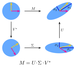
In linear algebra, the singular value decomposition (SVD) is a factorization of a real or complex matrix that generalizes the eigendecomposition of a square normal matrix to any matrix via an extension of the polar decomposition.
In mechanics and geometry, the 3D rotation group, often denoted SO(3), is the group of all rotations about the origin of three-dimensional Euclidean space under the operation of composition. By definition, a rotation about the origin is a transformation that preserves the origin, Euclidean distance, and orientation. Every non-trivial rotation is determined by its axis of rotation and its angle of rotation. Composing two rotations results in another rotation; every rotation has a unique inverse rotation; and the identity map satisfies the definition of a rotation. Owing to the above properties, the set of all rotations is a group under composition. Rotations are not commutative, making it a nonabelian group. Moreover, the rotation group has a natural structure as a manifold for which the group operations are smoothly differentiable; so it is in fact a Lie group. It is compact and has dimension 3.
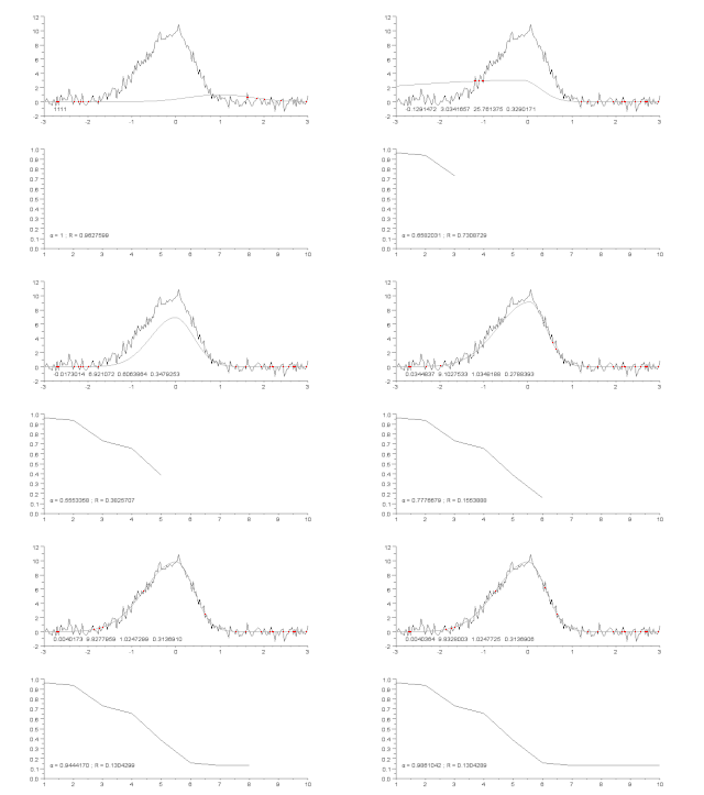
In mathematics and computing, the Levenberg–Marquardt algorithm, also known as the damped least-squares (DLS) method, is used to solve non-linear least squares problems. These minimization problems arise especially in least squares curve fitting.

Tikhonov regularization, named for Andrey Tikhonov, is a method of regularization of ill-posed problems. A special case of Tikhonov regularization, known as ridge regression, is particularly useful to mitigate the problem of multicollinearity in linear regression, which commonly occurs in models with large numbers of parameters. In general, the method provides improved efficiency in parameter estimation problems in exchange for a tolerable amount of bias.

In applied statistics, total least squares is a type of errors-in-variables regression, a least squares data modeling technique in which observational errors on both dependent and independent variables are taken into account. It is a generalization of Deming regression and also of orthogonal regression, and can be applied to both linear and non-linear models.
In statistics, a confidence region is a multi-dimensional generalization of a confidence interval. It is a set of points in an n-dimensional space, often represented as an ellipsoid around a point which is an estimated solution to a problem, although other shapes can occur.

The Gauss–Newton algorithm is used to solve non-linear least squares problems. It is a modification of Newton's method for finding a minimum of a function. Unlike Newton's method, the Gauss–Newton algorithm can only be used to minimize a sum of squared function values, but it has the advantage that second derivatives, which can be challenging to compute, are not required.

In statistics, ordinary least squares (OLS) is a type of linear least squares method for estimating the unknown parameters in a linear regression model. OLS chooses the parameters of a linear function of a set of explanatory variables by the principle of least squares: minimizing the sum of the squares of the differences between the observed dependent variable in the given dataset and those predicted by the linear function.
Weighted least squares (WLS), also known as weighted linear regression, is a generalization of ordinary least squares and linear regression in which the errors covariance matrix is allowed to be different from an identity matrix. WLS is also a specialization of generalized least squares in which the above matrix is diagonal.
Numerical linear algebra, sometimes called applied linear algebra, is the study of how matrix operations can be used to create computer algorithms which efficiently and accurately provide approximate answers to questions in continuous mathematics. It is a subfield of numerical analysis, and a type of linear algebra. Computers use floating-point arithmetic and cannot exactly represent irrational data, so when a computer algorithm is applied to a matrix of data, it can sometimes increase the difference between a number stored in the computer and the true number that it is an approximation of. Numerical linear algebra uses properties of vectors and matrices to develop computer algorithms that minimize the error introduced by the computer, and is also concerned with ensuring that the algorithm is as efficient as possible.

In statistics, Bayesian linear regression is an approach to linear regression in which the statistical analysis is undertaken within the context of Bayesian inference. When the regression model has errors that have a normal distribution, and if a particular form of prior distribution is assumed, explicit results are available for the posterior probability distributions of the model's parameters.

In statistics, Bayesian multivariate linear regression is a Bayesian approach to multivariate linear regression, i.e. linear regression where the predicted outcome is a vector of correlated random variables rather than a single scalar random variable. A more general treatment of this approach can be found in the article MMSE estimator.
In statistics, the projection matrix, sometimes also called the influence matrix or hat matrix, maps the vector of response values to the vector of fitted values. It describes the influence each response value has on each fitted value. The diagonal elements of the projection matrix are the leverages, which describe the influence each response value has on the fitted value for that same observation.

Non-linear least squares is the form of least squares analysis used to fit a set of m observations with a model that is non-linear in n unknown parameters (m ≥ n). It is used in some forms of nonlinear regression. The basis of the method is to approximate the model by a linear one and to refine the parameters by successive iterations. There are many similarities to linear least squares, but also some significant differences. In economic theory, the non-linear least squares method is applied in (i) the probit regression, (ii) threshold regression, (iii) smooth regression, (iv) logistic link regression, (v) Box-Cox transformed regressors.

In statistics, principal component regression (PCR) is a regression analysis technique that is based on principal component analysis (PCA). More specifically, PCR is used for estimating the unknown regression coefficients in a standard linear regression model.
The purpose of this page is to provide supplementary materials for the ordinary least squares article, reducing the load of the main article with mathematics and improving its accessibility, while at the same time retaining the completeness of exposition.

Linear least squares (LLS) is the least squares approximation of linear functions to data. It is a set of formulations for solving statistical problems involved in linear regression, including variants for ordinary (unweighted), weighted, and generalized (correlated) residuals. Numerical methods for linear least squares include inverting the matrix of the normal equations and orthogonal decomposition methods.


