Order of approximation

Last updated

In science, engineering, and other quantitative disciplines, order of approximation refers to formal or informal expressions for how accurate an approximation is.

Contents

Usage in science and engineering

In formal expressions, the ordinal number used before the word order refers to the highest power in the series expansion used in the approximation. The expressions: a zeroth-order approximation, a first-order approximation, a second-order approximation, and so forth are used as fixed phrases. The expression a zero-order approximation is also common. Cardinal numerals are occasionally used in expressions like an order-zero approximation, an order-one approximation, etc.

The omission of the word order leads to phrases that have less formal meaning. Phrases like first approximation or to a first approximation may refer to a roughly approximate value of a quantity. [1] [2] The phrase to a zeroth approximation indicates a wild guess. [3] The expression order of approximation is sometimes informally used to mean the number of significant figures, in increasing order of accuracy, or to the order of magnitude. However, this may be confusing, as these formal expressions do not directly refer to the order of derivatives.

The choice of series expansion depends on the scientific method used to investigate a phenomenon. The expression order of approximation is expected to indicate progressively more refined approximations of a function in a specified interval. The choice of order of approximation depends on the research purpose. One may wish to simplify a known analytic expression to devise a new application or, on the contrary, try to fit a curve to data points. Higher order of approximation is not always more useful than the lower one. For example, if a quantity is constant within the whole interval, approximating it with a second-order Taylor series will not increase the accuracy.

In the case of a smooth function, the nth-order approximation is a polynomial of degree  n, which is obtained by truncating the Taylor series to this degree. The formal usage of order of approximation corresponds to the omission of some terms of the series used in the expansion (usually the higher terms). This affects accuracy. The error usually varies within the interval. Thus the numbers zeroth, first, second etc. used formally in the above meaning do not directly give information about percent error or significant figures.

Zeroth-order

Zeroth-order approximation is the term scientists use for a first rough answer. Many simplifying assumptions are made, and when a number is needed, an order-of-magnitude answer (or zero significant figures) is often given. For example, you might say "the town has a few thousand residents", when it has 3,914 people in actuality. This is also sometimes referred to as an order-of-magnitude approximation. The zero of "zeroth-order" represents the fact that even the only number given, "a few", is itself loosely defined.

A zeroth-order approximation of a function (that is, mathematically determining a formula to fit multiple data points) will be constant, or a flat line with no slope: a polynomial of degree 0. For example,

could be – if data point accuracy were reported – an approximate fit to the data, obtained by simply averaging the x values and the y values. However, data points represent results of measurements and they do differ from points in Euclidean geometry. Thus quoting an average value containing three significant digits in the output with just one significant digit in the input data could be recognized as an example of false precision. With the implied accuracy of the data points of ±0.5, the zeroth order approximation could at best yield the result for y of ~3.7 ± 2.0 in the interval of x from −0.5 to 2.5, considering the standard deviation.

If the data points are reported as

the zeroth-order approximation results in

The accuracy of the result justifies an attempt to derive a multiplicative function for that average, for example,

One should be careful though, because the multiplicative function will be defined for the whole interval. If only three data points are available, one has no knowledge about the rest of the interval, which may be a large part of it. This means that y could have another component which equals 0 at the ends and in the middle of the interval. A number of functions having this property are known, for example y = sin πx. Taylor series is useful and helps predict an analytic solution, but the approximation alone does not provide conclusive evidence.

First-order

First-order approximation is the term scientists use for a slightly better answer. [3] Some simplifying assumptions are made, and when a number is needed, an answer with only one significant figure is often given ("the town has 4×10³, or four thousand, residents"). In the case of a first-order approximation, at least one number given is exact. In the zeroth-order example above, the quantity "a few" was given, but in the first-order example, the number "4" is given.

A first-order approximation of a function (that is, mathematically determining a formula to fit multiple data points) will be a linear approximation, straight line with a slope: a polynomial of degree 1. For example:

is an approximate fit to the data. In this example there is a zeroth-order approximation that is the same as the first-order, but the method of getting there is different; i.e. a wild stab in the dark at a relationship happened to be as good as an "educated guess".

Second-order

Second-order approximation is the term scientists use for a decent-quality answer. Few simplifying assumptions are made, and when a number is needed, an answer with two or more significant figures ("the town has 3.9×10³, or thirty-nine hundred, residents") is generally given. In mathematical finance, second-order approximations are known as convexity corrections. As in the examples above, the term "2nd order" refers to the number of exact numerals given for the imprecise quantity. In this case, "3" and "9" are given as the two successive levels of precision, instead of simply the "4" from the first order, or "a few" from the zeroth order found in the examples above.

A second-order approximation of a function (that is, mathematically determining a formula to fit multiple data points) will be a quadratic polynomial, geometrically, a parabola: a polynomial of degree 2. For example:

is an approximate fit to the data. In this case, with only three data points, a parabola is an exact fit based on the data provided. However, the data points for most of the interval are not available, which advises caution (see "zeroth order").

Higher-order

While higher-order approximations exist and are crucial to a better understanding and description of reality, they are not typically referred to by number.

Continuing the above, a third-order approximation would be required to perfectly fit four data points, and so on. See polynomial interpolation.

Colloquial usage

These terms are also used colloquially by scientists and engineers to describe phenomena that can be neglected as not significant (e.g. "Of course the rotation of the Earth affects our experiment, but it's such a high-order effect that we wouldn't be able to measure it." or "At these velocities, relativity is a fourth-order effect that we only worry about at the annual calibration.") In this usage, the ordinality of the approximation is not exact, but is used to emphasize its insignificance; the higher the number used, the less important the effect. The terminology, in this context, represents a high level of precision required to account for an effect which is inferred to be very small when compared to the overall subject matter. The higher the order, the more precision is required to measure the effect, and therefore the smallness of the effect in comparison to the overall measurement.

See also

Related Research Articles

<span class="mw-page-title-main">Interpolation</span> Method for estimating new data within known data points

In the mathematical field of numerical analysis, interpolation is a type of estimation, a method of constructing (finding) new data points based on the range of a discrete set of known data points.

<span class="mw-page-title-main">B-spline</span> Spline function

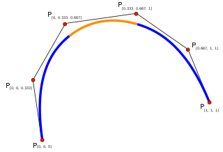
In the mathematical subfield of numerical analysis, a B-spline or basis spline is a spline function that has minimal support with respect to a given degree, smoothness, and domain partition. Any spline function of given degree can be expressed as a linear combination of B-splines of that degree. Cardinal B-splines have knots that are equidistant from each other. B-splines can be used for curve-fitting and numerical differentiation of experimental data.

In mathematics, a polynomial is an expression consisting of indeterminates and coefficients, that involves only the operations of addition, subtraction, multiplication, and non-negative integer exponentiation of variables. An example of a polynomial of a single indeterminate x is x2 − 4x + 7. An example in three variables is x3 + 2xyz2yz + 1.

<span class="mw-page-title-main">Differential calculus</span> Area of mathematics; subarea of calculus

In mathematics, differential calculus is a subfield of calculus that studies the rates at which quantities change. It is one of the two traditional divisions of calculus, the other being integral calculus—the study of the area beneath a curve.

<span class="mw-page-title-main">Taylor's theorem</span> Approximation of a function by a truncated power series

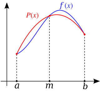
In calculus, Taylor's theorem gives an approximation of a k-times differentiable function around a given point by a polynomial of degree k, called the kth-order Taylor polynomial. For a smooth function, the Taylor polynomial is the truncation at the order k of the Taylor series of the function. The first-order Taylor polynomial is the linear approximation of the function, and the second-order Taylor polynomial is often referred to as the quadratic approximation. There are several versions of Taylor's theorem, some giving explicit estimates of the approximation error of the function by its Taylor polynomial.

In mathematics and computing, a root-finding algorithm is an algorithm for finding zeros, also called "roots", of continuous functions. A zero of a function f, from the real numbers to real numbers or from the complex numbers to the complex numbers, is a number x such that f(x) = 0. As, generally, the zeros of a function cannot be computed exactly nor expressed in closed form, root-finding algorithms provide approximations to zeros, expressed either as floating-point numbers or as small isolating intervals, or disks for complex roots.

<span class="mw-page-title-main">Linear interpolation</span> Method of curve fitting to construct new data points within the range of known data points

In mathematics, linear interpolation is a method of curve fitting using linear polynomials to construct new data points within the range of a discrete set of known data points.

<span class="mw-page-title-main">Numerical integration</span> Family of algorithms for finding the definite integral of a function

In analysis, numerical integration comprises a broad family of algorithms for calculating the numerical value of a definite integral, and by extension, the term is also sometimes used to describe the numerical solution of differential equations. This article focuses on calculation of definite integrals.

<span class="mw-page-title-main">Runge's phenomenon</span> Failure of convergence in interpolation

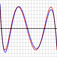
In the mathematical field of numerical analysis, Runge's phenomenon is a problem of oscillation at the edges of an interval that occurs when using polynomial interpolation with polynomials of high degree over a set of equispaced interpolation points. It was discovered by Carl David Tolmé Runge (1901) when exploring the behavior of errors when using polynomial interpolation to approximate certain functions. The discovery was important because it shows that going to higher degrees does not always improve accuracy. The phenomenon is similar to the Gibbs phenomenon in Fourier series approximations.

In numerical analysis, polynomial interpolation is the interpolation of a given data set by the polynomial of lowest possible degree that passes through the points of the dataset.

<span class="mw-page-title-main">Simpson's rule</span> Method for numerical integration

In numerical integration, Simpson's rules are several approximations for definite integrals, named after Thomas Simpson (1710–1761).

An approximation is anything that is intentionally similar but not exactly equal to something else.

In mathematics and statistics, a piecewise linear, PL or segmented function is a real-valued function of a real variable, whose graph is composed of straight-line segments.

<span class="mw-page-title-main">Spline (mathematics)</span> Mathematical function defined piecewise by polynomials

In mathematics, a spline is a special function defined piecewise by polynomials. In interpolating problems, spline interpolation is often preferred to polynomial interpolation because it yields similar results, even when using low degree polynomials, while avoiding Runge's phenomenon for higher degrees.

<span class="mw-page-title-main">Extrapolation</span> Method for estimating new data outside known data points

In mathematics, extrapolation is a type of estimation, beyond the original observation range, of the value of a variable on the basis of its relationship with another variable. It is similar to interpolation, which produces estimates between known observations, but extrapolation is subject to greater uncertainty and a higher risk of producing meaningless results. Extrapolation may also mean extension of a method, assuming similar methods will be applicable. Extrapolation may also apply to human experience to project, extend, or expand known experience into an area not known or previously experienced so as to arrive at a knowledge of the unknown. The extrapolation method can be applied in the interior reconstruction problem.

<span class="mw-page-title-main">Curve fitting</span> Process of constructing a curve that has the best fit to a series of data points

Curve fitting is the process of constructing a curve, or mathematical function, that has the best fit to a series of data points, possibly subject to constraints. Curve fitting can involve either interpolation, where an exact fit to the data is required, or smoothing, in which a "smooth" function is constructed that approximately fits the data. A related topic is regression analysis, which focuses more on questions of statistical inference such as how much uncertainty is present in a curve that is fit to data observed with random errors. Fitted curves can be used as an aid for data visualization, to infer values of a function where no data are available, and to summarize the relationships among two or more variables. Extrapolation refers to the use of a fitted curve beyond the range of the observed data, and is subject to a degree of uncertainty since it may reflect the method used to construct the curve as much as it reflects the observed data.

<span class="mw-page-title-main">Approximation theory</span> Theory of getting acceptably close inexact mathematical calculations

In mathematics, approximation theory is concerned with how functions can best be approximated with simpler functions, and with quantitatively characterizing the errors introduced thereby. Note that what is meant by best and simpler will depend on the application.

<span class="mw-page-title-main">Savitzky–Golay filter</span> Algorithm to smooth data points

A Savitzky–Golay filter is a digital filter that can be applied to a set of digital data points for the purpose of smoothing the data, that is, to increase the precision of the data without distorting the signal tendency. This is achieved, in a process known as convolution, by fitting successive sub-sets of adjacent data points with a low-degree polynomial by the method of linear least squares. When the data points are equally spaced, an analytical solution to the least-squares equations can be found, in the form of a single set of "convolution coefficients" that can be applied to all data sub-sets, to give estimates of the smoothed signal, at the central point of each sub-set. The method, based on established mathematical procedures, was popularized by Abraham Savitzky and Marcel J. E. Golay, who published tables of convolution coefficients for various polynomials and sub-set sizes in 1964. Some errors in the tables have been corrected. The method has been extended for the treatment of 2- and 3-dimensional data.

Clenshaw–Curtis quadrature and Fejér quadrature are methods for numerical integration, or "quadrature", that are based on an expansion of the integrand in terms of Chebyshev polynomials. Equivalently, they employ a change of variables and use a discrete cosine transform (DCT) approximation for the cosine series. Besides having fast-converging accuracy comparable to Gaussian quadrature rules, Clenshaw–Curtis quadrature naturally leads to nested quadrature rules, which is important for both adaptive quadrature and multidimensional quadrature (cubature).

In numerical analysis, Gauss–Legendre quadrature is a form of Gaussian quadrature for approximating the definite integral of a function. For integrating over the interval [−1, 1], the rule takes the form:

References

  1. first approximation in Webster's Third New International Dictionary, Könemann, ISBN   3-8290-5292-8.
  2. to a first approximation in Online Dictionary and Translations Webster-dictionary.org.
  3. 1 2 to a zeroth approximation in Online Dictionary and Translations Webster-dictionary.org.