Panel data

Last updated January 11, 2024

In statistics and econometrics, panel data and longitudinal data^[1]^[2] are both multi-dimensional data involving measurements over time. Panel data is a subset of longitudinal data where observations are for the same subjects each time.

Time series and cross-sectional data can be thought of as special cases of panel data that are in one dimension only (one panel member or individual for the former, one time point for the latter). A literature search often involves time series, cross-sectional, or panel data. Cross-panel data (CPD) is an innovative yet underappreciated source of information in the mathematical and statistical sciences. CPD stands out from other research methods because it vividly illustrates how independent and dependent variables may shift between countries. This panel data collection allows researchers to examine the connection between variables across several cross-sections and time periods and analyze the results of policy actions in other nations.^[3]

A study that uses panel data is called a longitudinal study or panel study.

Example

MRPP balanced panel
person	year	income	age	sex
1	2016	1300	27	1
1	2017	1600	28	1
1	2018	2000	29	1
2	2016	2000	38	2
2	2017	2300	39	2
2	2018	2400	40	2

MRPP unbalanced panel
person	year	income	age	sex
1	2016	1600	23	1
1	2017	1500	24	1
2	2016	1900	41	2
2	2017	2000	42	2
2	2018	2100	43	2
3	2017	3300	34	1

In the multiple response permutation procedure (MRPP) example above, two datasets with a panel structure are shown and the objective is to test whether there's a significant difference between people in the sample data. Individual characteristics (income, age, sex) are collected for different persons and different years. In the first dataset, two persons (1, 2) are observed every year for three years (2016, 2017, 2018). In the second dataset, three persons (1, 2, 3) are observed two times (person 1), three times (person 2), and one time (person 3), respectively, over three years (2016, 2017, 2018); in particular, person 1 is not observed in year 2018 and person 3 is not observed in 2016 or 2018.

A balanced panel (e.g., the first dataset above) is a dataset in which each panel member (i.e., person) is observed every year. Consequently, if a balanced panel contains $N$ panel members and $T$ periods, the number of observations ( $n$ ) in the dataset is necessarily $n=N\cdot T$ .

An unbalanced panel (e.g., the second dataset above) is a dataset in which at least one panel member is not observed every period. Therefore, if an unbalanced panel contains $N$ panel members and $T$ periods, then the following strict inequality holds for the number of observations ( $n$ ) in the dataset: $n<N\cdot T$ .

Both datasets above are structured in the long format, which is where one row holds one observation per time. Another way to structure panel data would be the wide format where one row represents one observational unit for all points in time (for the example, the wide format would have only two (first example) or three (second example) rows of data with additional columns for each time-varying variable (income, age).

Analysis

A panel has the form

X_{it},\quad i=1,\dots ,N,\quad t=1,\dots ,T,

where $i$ is the individual dimension and $t$ is the time dimension. A general panel data regression model is written as $y_{it}=\alpha +\beta 'X_{it}+u_{it}$ . Different assumptions can be made on the precise structure of this general model. Two important models are the fixed effects model and the random effects model.

Consider a generic panel data model:

y_{it}=\alpha +\beta 'X_{it}+u_{it},

u_{it}=\mu _{i}+v_{it}.

$\mu _{i}$ are individual-specific, time-invariant effects (e.g., in a panel of countries this could include geography, climate, etc.) which are fixed over time, whereas $v_{it}$ is a time-varying random component.

If $\mu _{i}$ is unobserved, and correlated with at least one of the independent variables, then it will cause omitted variable bias in a standard OLS regression. However, panel data methods, such as the fixed effects estimator or alternatively, the first-difference estimator can be used to control for it.

If $\mu _{i}$ is not correlated with any of the independent variables, ordinary least squares linear regression methods can be used to yield unbiased and consistent estimates of the regression parameters. However, because $\mu _{i}$ is fixed over time, it will induce serial correlation in the error term of the regression. This means that more efficient estimation techniques are available. Random effects is one such method: it is a special case of feasible generalized least squares which controls for the structure of the serial correlation induced by $\mu _{i}$ .

Dynamic panel data

Dynamic panel data describes the case where a lag of the dependent variable is used as regressor:

y_{it}=\alpha +\beta 'X_{it}+\gamma y_{it-1}+u_{it}.

The presence of the lagged dependent variable violates strict exogeneity, that is, endogeneity may occur. The fixed effect estimator and the first differences estimator both rely on the assumption of strict exogeneity. Hence, if $u_{i}$ is believed to be correlated with one of the independent variables, an alternative estimation technique must be used. Instrumental variables or GMM techniques are commonly used in this situation, such as the Arellano–Bond estimator.

Data sets which have a panel design

Russia Longitudinal Monitoring Survey (RLMS)
German Socio-Economic Panel (SOEP)
Household, Income and Labour Dynamics in Australia Survey (HILDA)
British Household Panel Survey (BHPS)
Survey of Family Income and Employment (SoFIE)
Survey of Income and Program Participation (SIPP)
Lifelong Labour Market Database (LLMDB)
Longitudinal Internet Studies for the Social sciences (LISS)
Panel Study of Income Dynamics (PSID)
Korean Labor and Income Panel Study (KLIPS)
China Family Panel Studies (CFPS)
German Family Panel (pairfam)
National Longitudinal Surveys (NLSY)
Labour Force Survey (LFS)
Korean Youth Panel (YP)
Korean Longitudinal Study of Aging (KLoSA)

Data sets which have a multi-dimensional panel design

Notes

↑ Diggle, Peter J.; Heagerty, Patrick; Liang, Kung-Yee; Zeger, Scott L. (2002). Analysis of Longitudinal Data (2nd ed.). Oxford University Press. p. 2. ISBN 0-19-852484-6.
↑ Fitzmaurice, Garrett M.; Laird, Nan M.; Ware, James H. (2004). Applied Longitudinal Analysis. Hoboken: John Wiley & Sons. p. 2. ISBN 0-471-21487-6.
↑ Zaman, Khalid (2023-01-24). "A Note on Cross-Panel Data Techniques". Latest Developments in Econometrics. 1 (1): 1–7. doi:10.5281/zenodo.7565625.

Related Research Articles

In statistics, maximum likelihood estimation (MLE) is a method of estimating the parameters of an assumed probability distribution, given some observed data. This is achieved by maximizing a likelihood function so that, under the assumed statistical model, the observed data is most probable. The point in the parameter space that maximizes the likelihood function is called the maximum likelihood estimate. The logic of maximum likelihood is both intuitive and flexible, and as such the method has become a dominant means of statistical inference.

In statistics and optimization, errors and residuals are two closely related and easily confused measures of the deviation of an observed value of an element of a statistical sample from its "true value". The error of an observation is the deviation of the observed value from the true value of a quantity of interest. The residual is the difference between the observed value and the estimated value of the quantity of interest. The distinction is most important in regression analysis, where the concepts are sometimes called the regression errors and regression residuals and where they lead to the concept of studentized residuals. In econometrics, "errors" are also called disturbances.

In statistical inference, specifically predictive inference, a prediction interval is an estimate of an interval in which a future observation will fall, with a certain probability, given what has already been observed. Prediction intervals are often used in regression analysis.

In statistics, a generalized linear model (GLM) is a flexible generalization of ordinary linear regression. The GLM generalizes linear regression by allowing the linear model to be related to the response variable via a link function and by allowing the magnitude of the variance of each measurement to be a function of its predicted value.

In statistics, econometrics, epidemiology and related disciplines, the method of instrumental variables (IV) is used to estimate causal relationships when controlled experiments are not feasible or when a treatment is not successfully delivered to every unit in a randomized experiment. Intuitively, IVs are used when an explanatory variable of interest is correlated with the error term (endogenous), in which case ordinary least squares and ANOVA give biased results. A valid instrument induces changes in the explanatory variable but has no independent effect on the dependent variable and is not correlated with the error term, allowing a researcher to uncover the causal effect of the explanatory variable on the dependent variable.

In statistics, omitted-variable bias (OVB) occurs when a statistical model leaves out one or more relevant variables. The bias results in the model attributing the effect of the missing variables to those that were included.

In statistics, ordinary least squares (OLS) is a type of linear least squares method for choosing the unknown parameters in a linear regression model by the principle of least squares: minimizing the sum of the squares of the differences between the observed dependent variable in the input dataset and the output of the (linear) function of the independent variable.

Panel (data) analysis is a statistical method, widely used in social science, epidemiology, and econometrics to analyze two-dimensional panel data. The data are usually collected over time and over the same individuals and then a regression is run over these two dimensions. Multidimensional analysis is an econometric method in which data are collected over more than two dimensions.

In statistics, a tobit model is any of a class of regression models in which the observed range of the dependent variable is censored in some way. The term was coined by Arthur Goldberger in reference to James Tobin, who developed the model in 1958 to mitigate the problem of zero-inflated data for observations of household expenditure on durable goods. Because Tobin's method can be easily extended to handle truncated and other non-randomly selected samples, some authors adopt a broader definition of the tobit model that includes these cases.

In statistics, the ordered logit model is an ordinal regression model—that is, a regression model for ordinal dependent variables—first considered by Peter McCullagh. For example, if one question on a survey is to be answered by a choice among "poor", "fair", "good", "very good" and "excellent", and the purpose of the analysis is to see how well that response can be predicted by the responses to other questions, some of which may be quantitative, then ordered logistic regression may be used. It can be thought of as an extension of the logistic regression model that applies to dichotomous dependent variables, allowing for more than two (ordered) response categories.

In statistics, ordered probit is a generalization of the widely used probit analysis to the case of more than two outcomes of an ordinal dependent variable. Similarly, the widely used logit method also has a counterpart ordered logit. Ordered probit, like ordered logit, is a particular method of ordinal regression.

In statistics, a fixed effects model is a statistical model in which the model parameters are fixed or non-random quantities. This is in contrast to random effects models and mixed models in which all or some of the model parameters are random variables. In many applications including econometrics and biostatistics a fixed effects model refers to a regression model in which the group means are fixed (non-random) as opposed to a random effects model in which the group means are a random sample from a population. Generally, data can be grouped according to several observed factors. The group means could be modeled as fixed or random effects for each grouping. In a fixed effects model each group mean is a group-specific fixed quantity.

In statistics, binomial regression is a regression analysis technique in which the response has a binomial distribution: it is the number of successes in a series of independent Bernoulli trials, where each trial has probability of success . In binomial regression, the probability of a success is related to explanatory variables: the corresponding concept in ordinary regression is to relate the mean value of the unobserved response to explanatory variables.

In statistics, a random effects model, also called a variance components model, is a statistical model where the model parameters are random variables. It is a kind of hierarchical linear model, which assumes that the data being analysed are drawn from a hierarchy of different populations whose differences relate to that hierarchy. A random effects model is a special case of a mixed model.

In econometrics, a multidimensional panel data is data of a phenomenon observed over three or more dimensions. This comes in contrast with panel data, observed over two dimensions. An example is a data set containing forecasts of one or multiple macroeconomic variables produced by multiple individuals, in multiple series at multiple times periods and for multiple horizons.

In statistics, errors-in-variables models or measurement error models are regression models that account for measurement errors in the independent variables. In contrast, standard regression models assume that those regressors have been measured exactly, or observed without error; as such, those models account only for errors in the dependent variables, or responses.

In statistics and econometrics, the first-difference (FD) estimator is an estimator used to address the problem of omitted variables with panel data. It is consistent under the assumptions of the fixed effects model. In certain situations it can be more efficient than the standard fixed effects estimator.

In econometrics, the Arellano–Bond estimator is a generalized method of moments estimator used to estimate dynamic models of panel data. It was proposed in 1991 by Manuel Arellano and Stephen Bond, based on the earlier work by Alok Bhargava and John Denis Sargan in 1983, for addressing certain endogeneity problems. The GMM-SYS estimator is a system that contains both the levels and the first difference equations. It provides an alternative to the standard first difference GMM estimator.

A partially linear model is a form of semiparametric model, since it contains parametric and nonparametric elements. Application of the least squares estimators is available to partially linear model, if the hypothesis of the known of nonparametric element is valid. Partially linear equations were first used in the analysis of the relationship between temperature and usage of electricity by Engle, Granger, Rice and Weiss (1986). Typical application of partially linear model in the field of Microeconomics is presented by Tripathi in the case of profitability of firm's production in 1997. Also, partially linear model applied successfully in some other academic field. In 1994, Zeger and Diggle introduced partially linear model into biometrics. In environmental science, Parda-Sanchez et al. used partially linear model to analysis collected data in 2000. So far, partially linear model was optimized in many other statistic methods. In 1988, Robinson applied Nadaraya-Waston kernel estimator to test the nonparametric element to build a least-squares estimator After that, in 1997, local linear method was found by Truong.

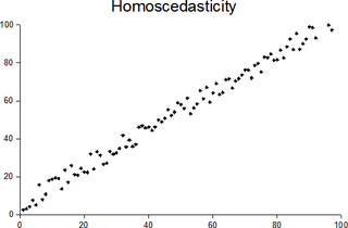
<span class="mw-page-title-main">Homoscedasticity and heteroscedasticity</span> Statistical property

In statistics, a sequence of random variables is homoscedastic if all its random variables have the same finite variance; this is also known as homogeneity of variance. The complementary notion is called heteroscedasticity, also known as heterogeneity of variance. The spellings homoskedasticity and heteroskedasticity are also frequently used. Assuming a variable is homoscedastic when in reality it is heteroscedastic results in unbiased but inefficient point estimates and in biased estimates of standard errors, and may result in overestimating the goodness of fit as measured by the Pearson coefficient.

References

Baltagi, Badi H. (2008). Econometric Analysis of Panel Data (Fourth ed.). Chichester: John Wiley & Sons. ISBN 978-0-470-51886-1.
Davies, A.; Lahiri, K. (1995). "A New Framework for Testing Rationality and Measuring Aggregate Shocks Using Panel Data". Journal of Econometrics . 68 (1): 205–227. doi:10.1016/0304-4076(94)01649-K.
Davies, A.; Lahiri, K. (2000). "Re-examining the Rational Expectations Hypothesis Using Panel Data on Multi-Period Forecasts". Analysis of Panels and Limited Dependent Variable Models. Cambridge: Cambridge University Press. pp. 226–254. ISBN 0-521-63169-6.
Frees, E. (2004). Longitudinal and Panel Data: Analysis and Applications in the Social Sciences. New York: Cambridge University Press. ISBN 0-521-82828-7.
Hsiao, Cheng (2003). Analysis of Panel Data (Second ed.). New York: Cambridge University Press. ISBN 0-521-52271-4.

External links

This page is based on this Wikipedia article
Text is available under the CC BY-SA 4.0 license; additional terms may apply.
Images, videos and audio are available under their respective licenses.

[1] Diggle, Peter J.; Heagerty, Patrick; Liang, Kung-Yee; Zeger, Scott L. (2002). Analysis of Longitudinal Data (2nd ed.). Oxford University Press. p. 2. ISBN 0-19-852484-6.

[2] Fitzmaurice, Garrett M.; Laird, Nan M.; Ware, James H. (2004). Applied Longitudinal Analysis. Hoboken: John Wiley & Sons. p. 2. ISBN 0-471-21487-6.

[3] Zaman, Khalid (2023-01-24). "A Note on Cross-Panel Data Techniques". Latest Developments in Econometrics. 1 (1): 1–7. doi:10.5281/zenodo.7565625.

[1]

[2]

[3]