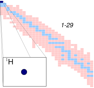
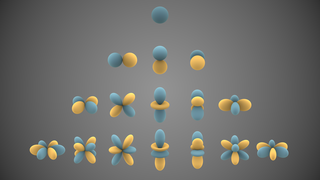
Hydrogen atomic orbitals of different energy levels. The more opaque areas are where one is most likely to find an electron at any given time.
In quantum mechanics, a spherically symmetric potential is a system of which the potential only depends on the radial distance from the spherical center and a location in space. A particle in a spherically symmetric potential will behave accordingly to said potential and can therefore be used as an approximation, for example, of the electron in a hydrogen atom or of the formation of chemical bonds.[1]
In the general time-independent case, the dynamics of a particle in a spherically symmetric potential are governed by a Hamiltonian of the following form:
Here, is the mass of the particle, is the momentum operator, and the potential depends only on the vector magnitude of the position vector, that is, the radial distance from the origin (hence the spherical symmetry of the problem).
To describe a particle in a spherically symmetric system, it is convenient to use spherical coordinates; denoted by , and . The time-independent Schrödinger equation for the system is then a separable, partial differential equation. This means solutions to the angular dimensions of the equation can be found independently of the radial dimension. This leaves an ordinary differential equation in terms only of the radius, , which determines the eigenstates for the particular potential, .
Since this equation holds for all values of , we get that , or that every angular momentum component commutes with the Hamiltonian.
Since and are such mutually commuting operators that also commute with the Hamiltonian, the wavefunctions can be expressed as or where is used to label different wavefunctions.
Since also commutes with the Hamiltonian, the energy eigenvalues in such cases are always independent of .
Combined with the fact that differential operators only act on the functions of and , it shows that if the solutions are assumed to be separable as , the radial wavefunction can always be chosen independent of values. Thus the wavefunction is expressed as:[2]
Solutions for potentials of interest
There are five cases of special importance:
, or solving the vacuum in the basis of spherical harmonics, which serves as the basis for other cases.
(finite) for and zero elsewhere.
for and infinite elsewhere, the spherical equivalent of the square well, useful to describe bound states in a nucleus or quantum dot.
for the three-dimensional isotropic harmonic oscillator.
The solutions of the Schrödinger equation in polar coordinates in vacuum are thus labelled by three quantum numbers: discrete indices ℓ and m, and k varying continuously in :
These solutions represent states of definite angular momentum, rather than of definite (linear) momentum, which are provided by plane waves .
Sphere with finite "square" potential
Consider the potential for and elsewhere - that is, inside a sphere of radius the potential is equal to and it is zero outside the sphere. A potential with such a finite discontinuity is called a square potential.[3]
We first consider bound states, i.e. states which display the particle mostly inside the box (confined states). Those have an energy less than the potential outside the sphere, i.e., they have negative energy. Also worth noticing is that unlike Coulomb potential, featuring an infinite number of discrete bound states, the spherical square well has only a finite (if any) number because of its finite range.
The resolution essentially follows that of the vacuum case above with normalization of the total wavefunction added, solving two Schrödinger equations — inside and outside the sphere — of the previous kind, i.e., with constant potential. The following constraints must hold for a normalizable, physical wavefunction:
The wavefunction must be regular at the origin.
The wavefunction and its derivative must be continuous at the potential discontinuity.
The wavefunction must converge at infinity.
The first constraint comes from the fact that Neumann and Hankel functions are singular at the origin. The physical requirement that must be defined everywhere selected Bessel function of the first kind over the other possibilities in the vacuum case. For the same reason, the solution will be of this kind inside the sphere:
Note that for bound states, . Bound states bring the novelty as compared to the vacuum case now that . This, along with the third constraint, selects the Hankel function of the first kind as the only converging solution at infinity (the singularity at the origin of these functions does not matter since we are now outside the sphere):
The second constraint on continuity of at along with normalization allows the determination of constants and . Continuity of the derivative (or logarithmic derivative for convenience) requires quantization of energy.
Sphere with infinite "square" potential
In case where the potential well is infinitely deep, so that we can take inside the sphere and outside, the problem becomes that of matching the wavefunction inside the sphere (the spherical Bessel functions) with identically zero wavefunction outside the sphere. Allowed energies are those for which the radial wavefunction vanishes at the boundary. Thus, we use the zeros of the spherical Bessel functions to find the energy spectrum and wavefunctions. Calling the kth zero of , we have:
so that the problem is reduced to the computations of these zeros , typically by using a table or calculator, as these zeros are not solvable for the general case.
In the special case (spherical symmetric orbitals), the spherical Bessel function is , which zeros can be easily given as . Their energy eigenvalues are thus:
i.e., is a non-negative integral number; is the (same) fundamental frequency of the modes of the oscillator. In this case , so that the radial Schrödinger equation becomes,
Introducing
and recalling that , we will show that the radial Schrödinger equation has the normalized solution,
First we transform the radial equation by a few successive substitutions to the generalized Laguerre differential equation, which has known solutions: the generalized Laguerre functions. Then we normalize the generalized Laguerre functions to unity. This normalization is with the usual volume element r2 dr.
Consideration of the limiting behavior of v(y) at the origin and at infinity suggests the following substitution for v(y),
This substitution transforms the differential equation to
where we divided through with , which can be done so long as y is not zero.
Transformation to Laguerre polynomials
If the substitution is used, , and the differential operators become
and
The expression between the square brackets multiplying becomes the differential equation characterizing the generalized Laguerre equation (see also Kummer's equation):
with .
Provided is a non-negative integral number, the solutions of this equations are generalized (associated) Laguerre polynomials
From the conditions on follows: (i) and (ii) and are either both odd or both even. This leads to the condition on given above.
Recovery of the normalized radial wavefunction
Remembering that , we get the normalized radial solution:
The normalization condition for the radial wave function is:
Other forms of the normalization constant can be derived by using properties of the gamma function, while noting that and are both of the same parity. This means that is always even, so that the gamma function becomes:
where we used the definition of the double factorial. Hence, the normalization constant is also given by:
A hydrogenic (hydrogen-like) atom is a two-particle system consisting of a nucleus and an electron. The two particles interact through the potential given by Coulomb's law:
r is the distance between the electron and the nucleus.
In order to simplify the Schrödinger equation, we introduce the following constants that define the atomic unit of energy and length:
where is the reduced mass in the limit. Substitute and into the radial Schrödinger equation given above. This gives an equation in which all natural constants are hidden,
Two classes of solutions of this equation exist:
(i) is negative, the corresponding eigenfunctions are square-integrable and the values of are quantized (discrete spectrum).
(ii) is non-negative, every real non-negative value of is physically allowed (continuous spectrum), the corresponding eigenfunctions are non-square integrable. Considering only class (i) solutions restricts the solutions to wavefunctions which are bound states, in contrast to the class (ii) solutions that are known as scattering states.
For class (i) solutions with negative W the quantity is real and positive. The scaling of , i.e., substitution of gives the Schrödinger equation:
For the inverse powers of x are negligible and the normalizable (and therefore, physical) solution for large is . Similarly, for the inverse square power dominates and the physical solution for small is xℓ+1. Hence, to obtain a full range solution we substitute
The equation for becomes,
Provided is a non-negative integer, this equation has polynomial solutions written as
A hydrogen atom is an atom of the chemical element hydrogen. The electrically neutral atom contains a single positively charged proton and a single negatively charged electron bound to the nucleus by the Coulomb force. Atomic hydrogen constitutes about 75% of the baryonic mass of the universe.
In mathematical physics and mathematics, the Pauli matrices are a set of three 2 × 2 complex matrices that are Hermitian, involutory and unitary. Usually indicated by the Greek letter sigma, they are occasionally denoted by tau when used in connection with isospin symmetries.
In mathematics and physics, Laplace's equation is a second-order partial differential equation named after Pierre-Simon Laplace, who first studied its properties. This is often written as
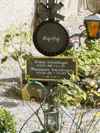
The Schrödinger equation is a linear partial differential equation that governs the wave function of a quantum-mechanical system. Its discovery was a significant landmark in the development of quantum mechanics. It is named after Erwin Schrödinger, who postulated the equation in 1925 and published it in 1926, forming the basis for the work that resulted in his Nobel Prize in Physics in 1933.
In statistics, maximum likelihood estimation (MLE) is a method of estimating the parameters of an assumed probability distribution, given some observed data. This is achieved by maximizing a likelihood function so that, under the assumed statistical model, the observed data is most probable. The point in the parameter space that maximizes the likelihood function is called the maximum likelihood estimate. The logic of maximum likelihood is both intuitive and flexible, and as such the method has become a dominant means of statistical inference.
In continuum mechanics, the infinitesimal strain theory is a mathematical approach to the description of the deformation of a solid body in which the displacements of the material particles are assumed to be much smaller than any relevant dimension of the body; so that its geometry and the constitutive properties of the material at each point of space can be assumed to be unchanged by the deformation.
In mathematics and physical science, spherical harmonics are special functions defined on the surface of a sphere. They are often employed in solving partial differential equations in many scientific fields. The table of spherical harmonics contains a list of common spherical harmonics.
In probability theory and statistics, the gamma distribution is a versatile two-parameter family of continuous probability distributions. The exponential distribution, Erlang distribution, and chi-squared distribution are special cases of the gamma distribution. There are two equivalent parameterizations in common use:
With a shape parameter k and a scale parameter θ
With a shape parameter and an inverse scale parameter , called a rate parameter.
In physics, a wave vector is a vector used in describing a wave, with a typical unit being cycle per metre. It has a magnitude and direction. Its magnitude is the wavenumber of the wave, and its direction is perpendicular to the wavefront. In isotropic media, this is also the direction of wave propagation.
In physics, the Hamilton–Jacobi equation, named after William Rowan Hamilton and Carl Gustav Jacob Jacobi, is an alternative formulation of classical mechanics, equivalent to other formulations such as Newton's laws of motion, Lagrangian mechanics and Hamiltonian mechanics.
In mathematics, the associated Legendre polynomials are the canonical solutions of the general Legendre equation
In mathematics, the Helmholtz equation is the eigenvalue problem for the Laplace operator. It corresponds to the linear partial differential equation:
In rotordynamics, the rigid rotor is a mechanical model of rotating systems. An arbitrary rigid rotor is a 3-dimensional rigid object, such as a top. To orient such an object in space requires three angles, known as Euler angles. A special rigid rotor is the linear rotor requiring only two angles to describe, for example of a diatomic molecule. More general molecules are 3-dimensional, such as water, ammonia, or methane.
In mathematics and physics, the Christoffel symbols are an array of numbers describing a metric connection. The metric connection is a specialization of the affine connection to surfaces or other manifolds endowed with a metric, allowing distances to be measured on that surface. In differential geometry, an affine connection can be defined without reference to a metric, and many additional concepts follow: parallel transport, covariant derivatives, geodesics, etc. also do not require the concept of a metric. However, when a metric is available, these concepts can be directly tied to the "shape" of the manifold itself; that shape is determined by how the tangent space is attached to the cotangent space by the metric tensor. Abstractly, one would say that the manifold has an associated (orthonormal) frame bundle, with each "frame" being a possible choice of a coordinate frame. An invariant metric implies that the structure group of the frame bundle is the orthogonal group O(p, q). As a result, such a manifold is necessarily a (pseudo-)Riemannian manifold. The Christoffel symbols provide a concrete representation of the connection of (pseudo-)Riemannian geometry in terms of coordinates on the manifold. Additional concepts, such as parallel transport, geodesics, etc. can then be expressed in terms of Christoffel symbols.
The theoretical and experimental justification for the Schrödinger equation motivates the discovery of the Schrödinger equation, the equation that describes the dynamics of nonrelativistic particles. The motivation uses photons, which are relativistic particles with dynamics described by Maxwell's equations, as an analogue for all types of particles.
The Gross–Pitaevskii equation describes the ground state of a quantum system of identical bosons using the Hartree–Fock approximation and the pseudopotential interaction model.
A hydrogen-like atom (or hydrogenic atom) is any atom or ion with a single valence electron. These atoms are isoelectronic with hydrogen. Examples of hydrogen-like atoms include, but are not limited to, hydrogen itself, all alkali metals such as Rb and Cs, singly ionized alkaline earth metals such as Ca+ and Sr+ and other ions such as He+, Li2+, and Be3+ and isotopes of any of the above. A hydrogen-like atom includes a positively charged core consisting of the atomic nucleus and any core electrons as well as a single valence electron. Because helium is common in the universe, the spectroscopy of singly ionized helium is important in EUV astronomy, for example, of DO white dwarf stars.
In mathematics, a Coulomb wave function is a solution of the Coulomb wave equation, named after Charles-Augustin de Coulomb. They are used to describe the behavior of charged particles in a Coulomb potential and can be written in terms of confluent hypergeometric functions or Whittaker functions of imaginary argument.
Curvilinear coordinates can be formulated in tensor calculus, with important applications in physics and engineering, particularly for describing transportation of physical quantities and deformation of matter in fluid mechanics and continuum mechanics.
In pure and applied mathematics, quantum mechanics and computer graphics, a tensor operator generalizes the notion of operators which are scalars and vectors. A special class of these are spherical tensor operators which apply the notion of the spherical basis and spherical harmonics. The spherical basis closely relates to the description of angular momentum in quantum mechanics and spherical harmonic functions. The coordinate-free generalization of a tensor operator is known as a representation operator.
↑ A. Messiah, Quantum Mechanics, vol. I, p. 78, North Holland Publishing Company, Amsterdam (1967). Translation from the French by G.M. Temmer
↑ H. Margenau and G. M. Murphy, The Mathematics of Physics and Chemistry, Van Nostrand, 2nd edition (1956), p. 130. Note that convention of the Laguerre polynomial in this book differs from the present one. If we indicate the Laguerre in the definition of Margenau and Murphy with a bar on top, we have .
This page is based on this Wikipedia article Text is available under the CC BY-SA 4.0 license; additional terms may apply. Images, videos and audio are available under their respective licenses.