In vector calculus, the gradient of a scalar-valued differentiable function of several variables is the vector field whose value at a point gives the direction and the rate of fastest increase. The gradient transforms like a vector under change of basis of the space of variables of . If the gradient of a function is non-zero at a point , the direction of the gradient is the direction in which the function increases most quickly from , and the magnitude of the gradient is the rate of increase in that direction, the greatest absolute directional derivative. Further, a point where the gradient is the zero vector is known as a stationary point. The gradient thus plays a fundamental role in optimization theory, where it is used to minimize a function by gradient descent. In coordinate-free terms, the gradient of a function may be defined by:
In vector calculus, the Jacobian matrix of a vector-valued function of several variables is the matrix of all its first-order partial derivatives. When this matrix is square, that is, when the function takes the same number of variables as input as the number of vector components of its output, its determinant is referred to as the Jacobian determinant. Both the matrix and the determinant are often referred to simply as the Jacobian in literature.

In Euclidean geometry, a translation is a geometric transformation that moves every point of a figure, shape or space by the same distance in a given direction. A translation can also be interpreted as the addition of a constant vector to every point, or as shifting the origin of the coordinate system. In a Euclidean space, any translation is an isometry.
Edge detection includes a variety of mathematical methods that aim at identifying edges, defined as curves in a digital image at which the image brightness changes sharply or, more formally, has discontinuities. The same problem of finding discontinuities in one-dimensional signals is known as step detection and the problem of finding signal discontinuities over time is known as change detection. Edge detection is a fundamental tool in image processing, machine vision and computer vision, particularly in the areas of feature detection and feature extraction.
In mathematics, the Hessian matrix, Hessian or Hesse matrix is a square matrix of second-order partial derivatives of a scalar-valued function, or scalar field. It describes the local curvature of a function of many variables. The Hessian matrix was developed in the 19th century by the German mathematician Ludwig Otto Hesse and later named after him. Hesse originally used the term "functional determinants". The Hessian is sometimes denoted by H or, ambiguously, by ∇2.

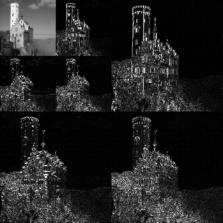
The Sobel operator, sometimes called the Sobel–Feldman operator or Sobel filter, is used in image processing and computer vision, particularly within edge detection algorithms where it creates an image emphasising edges. It is named after Irwin Sobel and Gary M. Feldman, colleagues at the Stanford Artificial Intelligence Laboratory (SAIL). Sobel and Feldman presented the idea of an "Isotropic 3 × 3 Image Gradient Operator" at a talk at SAIL in 1968. Technically, it is a discrete differentiation operator, computing an approximation of the gradient of the image intensity function. At each point in the image, the result of the Sobel–Feldman operator is either the corresponding gradient vector or the norm of this vector. The Sobel–Feldman operator is based on convolving the image with a small, separable, and integer-valued filter in the horizontal and vertical directions and is therefore relatively inexpensive in terms of computations. On the other hand, the gradient approximation that it produces is relatively crude, in particular for high-frequency variations in the image.
The Roberts cross operator is used in image processing and computer vision for edge detection. It was one of the first edge detectors and was initially proposed by Lawrence Roberts in 1963. As a differential operator, the idea behind the Roberts cross operator is to approximate the gradient of an image through discrete differentiation which is achieved by computing the sum of the squares of the differences between diagonally adjacent pixels.

The Canny edge detector is an edge detection operator that uses a multi-stage algorithm to detect a wide range of edges in images. It was developed by John F. Canny in 1986. Canny also produced a computational theory of edge detection explaining why the technique works.
In control engineering and system identification, a state-space representation is a mathematical model of a physical system specified as a set of input, output, and variables related by first-order differential equations or difference equations. Such variables, called state variables, evolve over time in a way that depends on the values they have at any given instant and on the externally imposed values of input variables. Output variables’ values depend on the state variable values and may also depend on the input variable values.
In numerical analysis and functional analysis, a discrete wavelet transform (DWT) is any wavelet transform for which the wavelets are discretely sampled. As with other wavelet transforms, a key advantage it has over Fourier transforms is temporal resolution: it captures both frequency and location information.
The scale-invariant feature transform (SIFT) is a computer vision algorithm to detect, describe, and match local features in images, invented by David Lowe in 1999. Applications include object recognition, robotic mapping and navigation, image stitching, 3D modeling, gesture recognition, video tracking, individual identification of wildlife and match moving.
In signal processing, the Wiener filter is a filter used to produce an estimate of a desired or target random process by linear time-invariant (LTI) filtering of an observed noisy process, assuming known stationary signal and noise spectra, and additive noise. The Wiener filter minimizes the mean square error between the estimated random process and the desired process.
In mathematics, the discrete Laplace operator is an analog of the continuous Laplace operator, defined so that it has meaning on a graph or a discrete grid. For the case of a finite-dimensional graph, the discrete Laplace operator is more commonly called the Laplacian matrix.
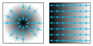
An image gradient is a directional change in the intensity or color in an image. The gradient of the image is one of the fundamental building blocks in image processing. For example, the Canny edge detector uses image gradient for edge detection. In graphics software for digital image editing, the term gradient or color gradient is also used for a gradual blend of color which can be considered as an even gradation from low to high values, as used from white to black in the images to the right. Another name for this is color progression.
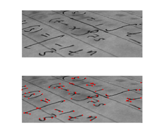
Corner detection is an approach used within computer vision systems to extract certain kinds of features and infer the contents of an image. Corner detection is frequently used in motion detection, image registration, video tracking, image mosaicing, panorama stitching, 3D reconstruction and object recognition. Corner detection overlaps with the topic of interest point detection.
In image processing, ridge detection is the attempt, via software, to locate ridges in an image, defined as curves whose points are local maxima of the function, akin to geographical ridges.
The Kirsch operator or Kirsch compass kernel is a non-linear edge detector that finds the maximum edge strength in a few predetermined directions. It is named after the computer scientist Russell Kirsch.
The principal curvature-based region detector, also called PCBR is a feature detector used in the fields of computer vision and image analysis. Specifically the PCBR detector is designed for object recognition applications.
Chessboards arise frequently in computer vision theory and practice because their highly structured geometry is well-suited for algorithmic detection and processing. The appearance of chessboards in computer vision can be divided into two main areas: camera calibration and feature extraction. This article provides a unified discussion of the role that chessboards play in the canonical methods from these two areas, including references to the seminal literature, examples, and pointers to software implementations.

Gradient vector flow (GVF), a computer vision framework introduced by Chenyang Xu and Jerry L. Prince, is the vector field that is produced by a process that smooths and diffuses an input vector field. It is usually used to create a vector field from images that points to object edges from a distance. It is widely used in image analysis and computer vision applications for object tracking, shape recognition, segmentation, and edge detection. In particular, it is commonly used in conjunction with active contour model.


