In probability theory, the expected value is a generalization of the weighted average. Informally, the expected value is the arithmetic mean of the possible values a random variable can take, weighted by the probability of those outcomes. Since it is obtained through arithmetic, the expected value sometimes may not even be included in the sample data set; it is not the value you would "expect" to get in reality.
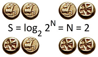
In information theory, the entropy of a random variable is the average level of "information", "surprise", or "uncertainty" inherent to the variable's possible outcomes. Given a discrete random variable , which takes values in the alphabet and is distributed according to :
Probability theory or probability calculus is the branch of mathematics concerned with probability. Although there are several different probability interpretations, probability theory treats the concept in a rigorous mathematical manner by expressing it through a set of axioms. Typically these axioms formalise probability in terms of a probability space, which assigns a measure taking values between 0 and 1, termed the probability measure, to a set of outcomes called the sample space. Any specified subset of the sample space is called an event.
In probability theory and statistics, a probability distribution is the mathematical function that gives the probabilities of occurrence of different possible outcomes for an experiment. It is a mathematical description of a random phenomenon in terms of its sample space and the probabilities of events.
A random variable is a mathematical formalization of a quantity or object which depends on random events. The term 'random variable' can be misleading as its mathematical definition is not actually random nor a variable, but rather it is a function from possible outcomes in a sample space to a measurable space, often to the real numbers.
In probability theory, a probability space or a probability triple is a mathematical construct that provides a formal model of a random process or "experiment". For example, one can define a probability space which models the throwing of a die.

In probability theory, a probability density function (PDF), density function, or density of an absolutely continuous random variable, is a function whose value at any given sample in the sample space can be interpreted as providing a relative likelihood that the value of the random variable would be equal to that sample. Probability density is the probability per unit length, in other words, while the absolute likelihood for a continuous random variable to take on any particular value is 0, the value of the PDF at two different samples can be used to infer, in any particular draw of the random variable, how much more likely it is that the random variable would be close to one sample compared to the other sample.
In probability and statistics, a Bernoulli process is a finite or infinite sequence of binary random variables, so it is a discrete-time stochastic process that takes only two values, canonically 0 and 1. The component Bernoulli variablesXi are identically distributed and independent. Prosaically, a Bernoulli process is a repeated coin flipping, possibly with an unfair coin. Every variable Xi in the sequence is associated with a Bernoulli trial or experiment. They all have the same Bernoulli distribution. Much of what can be said about the Bernoulli process can also be generalized to more than two outcomes ; this generalization is known as the Bernoulli scheme.

In probability theory and statistics, the Bernoulli distribution, named after Swiss mathematician Jacob Bernoulli, is the discrete probability distribution of a random variable which takes the value 1 with probability and the value 0 with probability . Less formally, it can be thought of as a model for the set of possible outcomes of any single experiment that asks a yes–no question. Such questions lead to outcomes that are boolean-valued: a single bit whose value is success/yes/true/one with probability p and failure/no/false/zero with probability q. It can be used to represent a coin toss where 1 and 0 would represent "heads" and "tails", respectively, and p would be the probability of the coin landing on heads. In particular, unfair coins would have

In statistics, the logistic model is a statistical model that models the log-odds of an event as a linear combination of one or more independent variables. In regression analysis, logistic regression is estimating the parameters of a logistic model. Formally, in binary logistic regression there is a single binary dependent variable, coded by an indicator variable, where the two values are labeled "0" and "1", while the independent variables can each be a binary variable or a continuous variable. The corresponding probability of the value labeled "1" can vary between 0 and 1, hence the labeling; the function that converts log-odds to probability is the logistic function, hence the name. The unit of measurement for the log-odds scale is called a logit, from logistic unit, hence the alternative names. See § Background and § Definition for formal mathematics, and § Example for a worked example.
In mathematics, the moments of a function are certain quantitative measures related to the shape of the function's graph. If the function represents mass density, then the zeroth moment is the total mass, the first moment is the center of mass, and the second moment is the moment of inertia. If the function is a probability distribution, then the first moment is the expected value, the second central moment is the variance, the third standardized moment is the skewness, and the fourth standardized moment is the kurtosis. The mathematical concept is closely related to the concept of moment in physics.
In probability theory and statistics, the conditional probability distribution is a probability distribution that describes the probability of an outcome given the occurrence of a particular event. Given two jointly distributed random variables and , the conditional probability distribution of given is the probability distribution of when is known to be a particular value; in some cases the conditional probabilities may be expressed as functions containing the unspecified value of as a parameter. When both and are categorical variables, a conditional probability table is typically used to represent the conditional probability. The conditional distribution contrasts with the marginal distribution of a random variable, which is its distribution without reference to the value of the other variable.
In probability and statistics, a mixture distribution is the probability distribution of a random variable that is derived from a collection of other random variables as follows: first, a random variable is selected by chance from the collection according to given probabilities of selection, and then the value of the selected random variable is realized. The underlying random variables may be random real numbers, or they may be random vectors, in which case the mixture distribution is a multivariate distribution.

Given two random variables that are defined on the same probability space, the joint probability distribution is the corresponding probability distribution on all possible pairs of outputs. The joint distribution can just as well be considered for any given number of random variables. The joint distribution encodes the marginal distributions, i.e. the distributions of each of the individual random variables and the conditional probability distributions, which deal with how the outputs of one random variable are distributed when given information on the outputs of the other random variable(s).
This glossary of statistics and probability is a list of definitions of terms and concepts used in the mathematical sciences of statistics and probability, their sub-disciplines, and related fields. For additional related terms, see Glossary of mathematics and Glossary of experimental design.
In mathematics, the Bernoulli scheme or Bernoulli shift is a generalization of the Bernoulli process to more than two possible outcomes. Bernoulli schemes appear naturally in symbolic dynamics, and are thus important in the study of dynamical systems. Many important dynamical systems exhibit a repellor that is the product of the Cantor set and a smooth manifold, and the dynamics on the Cantor set are isomorphic to that of the Bernoulli shift. This is essentially the Markov partition. The term shift is in reference to the shift operator, which may be used to study Bernoulli schemes. The Ornstein isomorphism theorem shows that Bernoulli shifts are isomorphic when their entropy is equal.
In probability theory, random element is a generalization of the concept of random variable to more complicated spaces than the simple real line. The concept was introduced by Maurice Fréchet (1948) who commented that the “development of probability theory and expansion of area of its applications have led to necessity to pass from schemes where (random) outcomes of experiments can be described by number or a finite set of numbers, to schemes where outcomes of experiments represent, for example, vectors, functions, processes, fields, series, transformations, and also sets or collections of sets.”
This article discusses how information theory is related to measure theory.
In probability theory and statistics, a categorical distribution is a discrete probability distribution that describes the possible results of a random variable that can take on one of K possible categories, with the probability of each category separately specified. There is no innate underlying ordering of these outcomes, but numerical labels are often attached for convenience in describing the distribution,. The K-dimensional categorical distribution is the most general distribution over a K-way event; any other discrete distribution over a size-K sample space is a special case. The parameters specifying the probabilities of each possible outcome are constrained only by the fact that each must be in the range 0 to 1, and all must sum to 1.
In probability theory and statistics, the law of the unconscious statistician, or LOTUS, is a theorem which expresses the expected value of a function g(X) of a random variable X in terms of g and the probability distribution of X.