
In physics and geometry, a catenary is the curve that an idealized hanging chain or cable assumes under its own weight when supported only at its ends in a uniform gravitational field.
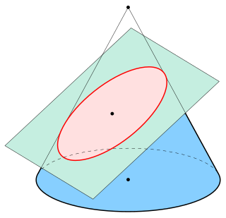
In mathematics, an ellipse is a plane curve surrounding two focal points, such that for all points on the curve, the sum of the two distances to the focal points is a constant. It generalizes a circle, which is the special type of ellipse in which the two focal points are the same. The elongation of an ellipse is measured by its eccentricity , a number ranging from to .
In classical mechanics, a harmonic oscillator is a system that, when displaced from its equilibrium position, experiences a restoring force F proportional to the displacement x:

In mathematics, a hyperbola is a type of smooth curve lying in a plane, defined by its geometric properties or by equations for which it is the solution set. A hyperbola has two pieces, called connected components or branches, that are mirror images of each other and resemble two infinite bows. The hyperbola is one of the three kinds of conic section, formed by the intersection of a plane and a double cone. If the plane intersects both halves of the double cone but does not pass through the apex of the cones, then the conic is a hyperbola.
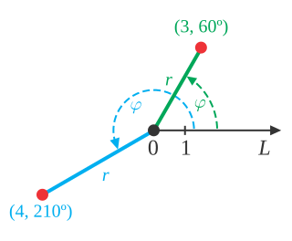
In mathematics, the polar coordinate system is a two-dimensional coordinate system in which each point on a plane is determined by a distance from a reference point and an angle from a reference direction. The reference point is called the pole, and the ray from the pole in the reference direction is the polar axis. The distance from the pole is called the radial coordinate, radial distance or simply radius, and the angle is called the angular coordinate, polar angle, or azimuth. Angles in polar notation are generally expressed in either degrees or radians.

The Navier–Stokes equations are partial differential equations which describe the motion of viscous fluid substances. They were named after French engineer and physicist Claude-Louis Navier and the Irish physicist and mathematician George Gabriel Stokes. They were developed over several decades of progressively building the theories, from 1822 (Navier) to 1842–1850 (Stokes).

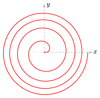
A hyperbolic spiral is a type of spiral with a pitch angle that increases with distance from its center, unlike the constant angles of logarithmic spirals or decreasing angles of Archimedean spirals. As this curve widens, it approaches an asymptotic line. It can be found in the view up a spiral staircase and the starting arrangement of certain footraces, and is used to model spiral galaxies and architectural volutes.
A Fermat's spiral or parabolic spiral is a plane curve with the property that the area between any two consecutive full turns around the spiral is invariant. As a result, the distance between turns grows in inverse proportion to their distance from the spiral center, contrasting with the Archimedean spiral and the logarithmic spiral. Fermat spirals are named after Pierre de Fermat.

In mathematics, the inverse trigonometric functions are the inverse functions of the trigonometric functions. Specifically, they are the inverses of the sine, cosine, tangent, cotangent, secant, and cosecant functions, and are used to obtain an angle from any of the angle's trigonometric ratios. Inverse trigonometric functions are widely used in engineering, navigation, physics, and geometry.

In geometry, the subtangent and related terms are certain line segments defined using the line tangent to a curve at a given point and the coordinate axes. The terms are somewhat archaic today but were in common use until the early part of the 20th century.
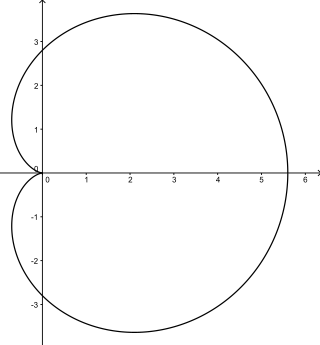
In geometry, a cardioid is a plane curve traced by a point on the perimeter of a circle that is rolling around a fixed circle of the same radius. It can also be defined as an epicycloid having a single cusp. It is also a type of sinusoidal spiral, and an inverse curve of the parabola with the focus as the center of inversion. A cardioid can also be defined as the set of points of reflections of a fixed point on a circle through all tangents to the circle.
In trigonometry, tangent half-angle formulas relate the tangent of half of an angle to trigonometric functions of the entire angle. The tangent of half an angle is the stereographic projection of the circle through the point at angle onto the line through the angles . Among these formulas are the following:

In probability theory, a distribution is said to be stable if a linear combination of two independent random variables with this distribution has the same distribution, up to location and scale parameters. A random variable is said to be stable if its distribution is stable. The stable distribution family is also sometimes referred to as the Lévy alpha-stable distribution, after Paul Lévy, the first mathematician to have studied it.
In general relativity, Schwarzschild geodesics describe the motion of test particles in the gravitational field of a central fixed mass that is, motion in the Schwarzschild metric. Schwarzschild geodesics have been pivotal in the validation of Einstein's theory of general relativity. For example, they provide accurate predictions of the anomalous precession of the planets in the Solar System and of the deflection of light by gravity.

Arc length is the distance between two points along a section of a curve.
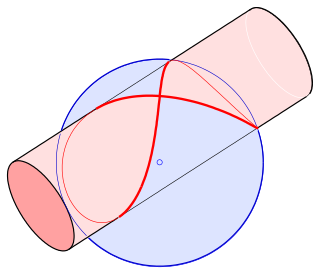
In mathematics, Viviani's curve, also known as Viviani's window, is a figure eight shaped space curve named after the Italian mathematician Vincenzo Viviani. It is the intersection of a sphere with a cylinder that is tangent to the sphere and passes through two poles of the sphere. Before Viviani this curve was studied by Simon de La Loubère and Gilles de Roberval.

The Duffing equation, named after Georg Duffing (1861–1944), is a non-linear second-order differential equation used to model certain damped and driven oscillators. The equation is given by
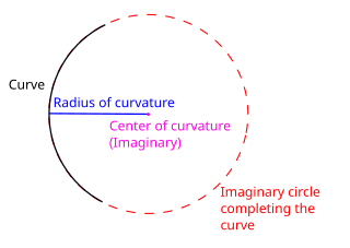
In differential geometry, the radius of curvature, R, is the reciprocal of the curvature. For a curve, it equals the radius of the circular arc which best approximates the curve at that point. For surfaces, the radius of curvature is the radius of a circle that best fits a normal section or combinations thereof.

In the geometry of curves, an orthoptic is the set of points for which two tangents of a given curve meet at a right angle.

In mathematics, a conical spiral, also known as a conical helix, is a space curve on a right circular cone, whose floor projection is a plane spiral. If the floor projection is a logarithmic spiral, it is called conchospiral.


