A slowly changing dimension (SCD) in data management and data warehousing is a dimension which contains relatively static data which can change slowly but unpredictably, rather than according to a regular schedule.[1] Some examples of typical slowly changing dimensions are entities such as names of geographical locations, customers, or products.
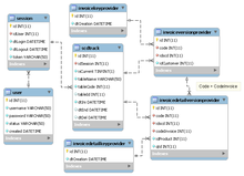
For example, a database may contain a fact table that stores sales records. This fact table would be linked to dimensions by means of foreign keys. One of these dimensions may contain data about the company's salespeople: e.g., the regional offices in which they work. However, the salespeople are sometimes transferred from one regional office to another. For historical sales reporting purposes it may be necessary to keep a record of the fact that a particular sales person had been assigned to a particular regional office at an earlier date, whereas that sales person is now assigned to a different regional office. Using SCD can help solve this issue.
Dealing with these issues involves SCD management methodologies referred to as Type 0 through 6. Type 6 SCDs are also sometimes called Hybrid SCDs.
Type 0: retain original
The Type 0 dimension attributes never change and are assigned to attributes that have durable values or are described as 'Original'. Examples: Date of Birth, Original Credit Score. Type 0 applies to most date dimension attributes.[2]
Type 1: overwrite
This method overwrites old with new data, and therefore does not track historical data.
Example of a supplier table:
Supplier_Key
Supplier_Code
Supplier_Name
Supplier_State
123
ABC
Acme Supply Co
CA
In the above example, Supplier_Code is the natural key and Supplier_Key is a surrogate key. Technically, the surrogate key is not necessary, since the row will be unique by the natural key (Supplier_Code).
If the supplier relocates the headquarters to Illinois the record would be overwritten:
Supplier_Key
Supplier_Code
Supplier_Name
Supplier_State
123
ABC
Acme Supply Co
IL
The disadvantage of the Type 1 method is that there is no history in the data warehouse. It has the advantage however that it's easy to maintain.
If one has calculated an aggregate table summarizing facts by supplier state, it will need to be recalculated when the Supplier_State is changed.[1]
Type 2: add new row
This method tracks historical data by creating multiple records for a given natural key in the dimensional tables with separate surrogate keys and/or different version numbers. Unlimited history is preserved for each insert. The natural key in these examples is the "Supplier_Code" of "ABC".
For example, if the supplier relocates to Illinois the version numbers will be incremented sequentially:
Supplier_Key
Supplier_Code
Supplier_Name
Supplier_State
Version
123
ABC
Acme Supply Co
CA
0
124
ABC
Acme Supply Co
IL
1
125
ABC
Acme Supply Co
NY
2
Another method is to add 'effective date' columns.
Supplier_Key
Supplier_Code
Supplier_Name
Supplier_State
Start_Date
End_Date
123
ABC
Acme Supply Co
CA
2000-01-01T00:00:00
2004-12-22T00:00:00
124
ABC
Acme Supply Co
IL
2004-12-22T00:00:00
NULL
The Start date/time of the second row is equal to the End date/time of the previous row. The null End_Date in row two indicates the current tuple version. A standardized surrogate high date (e.g. 9999-12-31) may instead be used as an end date, so that the field can be included in an index, and so that null-value substitution is not required when querying. In some database software, using an artificial high date value could cause performance issues, that using a null value would prevent.
And a third method uses an effective date and a current flag.
Supplier_Key
Supplier_Code
Supplier_Name
Supplier_State
Effective_Date
Current_Flag
123
ABC
Acme Supply Co
CA
2000-01-01T00:00:00
N
124
ABC
Acme Supply Co
IL
2004-12-22T00:00:00
Y
The Current_Flag value of 'Y' indicates the current tuple version.
Transactions that reference a particular surrogate key (Supplier_Key) are then permanently bound to the time slices defined by that row of the slowly changing dimension table. An aggregate table summarizing facts by supplier state continues to reflect the historical state, i.e. the state the supplier was in at the time of the transaction; no update is needed. To reference the entity via the natural key, it is necessary to remove the unique constraint making referential integrity by DBMS impossible.
If there are retroactive changes made to the contents of the dimension, or if new attributes are added to the dimension (for example a Sales_Rep column) which have different effective dates from those already defined, then this can result in the existing transactions needing to be updated to reflect the new situation. This can be an expensive database operation, so Type 2 SCDs are not a good choice if the dimensional model is subject to frequent change.[1]
Type 3: add new attribute
This method tracks changes using separate columns and preserves limited history. The Type 3 preserves limited history as it is limited to the number of columns designated for storing historical data. The original table structure in Type 1 and Type 2 is the same but Type 3 adds additional columns. In the following example, an additional column has been added to the table to record the supplier's original state - only the previous history is stored.
Supplier_Key
Supplier_Code
Supplier_Name
Original_Supplier_State
Effective_Date
Current_Supplier_State
123
ABC
Acme Supply Co
CA
2004-12-22T00:00:00
IL
This record contains a column for the original state and current state—cannot track the changes if the supplier relocates a second time.
One variation of this is to create the field Previous_Supplier_State instead of Original_Supplier_State which would track only the most recent historical change.[1]
Type 4: add history table
The Type 4 method is usually referred to as using "history tables", where one table keeps the current data, and an additional table is used to keep a record of some or all changes. Both the surrogate keys are referenced in the fact table to enhance query performance.
For the example below, the original table name is Supplier and the history table is Supplier_History:
Supplier
Supplier_Key
Supplier_Code
Supplier_Name
Supplier_State
124
ABC
Acme & Johnson Supply Co
IL
Supplier_History
Supplier_Key
Supplier_Code
Supplier_Name
Supplier_State
Create_Date
123
ABC
Acme Supply Co
CA
2003-06-14T00:00:00
124
ABC
Acme & Johnson Supply Co
IL
2004-12-22T00:00:00
This method resembles how database audit tables and change data capture techniques function.
Type 5
The type 5 technique builds on the type 4 mini-dimension by embedding a “current profile” mini-dimension key in the base dimension that's overwritten as a type 1 attribute. This approach is called type 5 because 4 + 1 equals 5. The type 5 slowly changing dimension allows the currently-assigned mini-dimension attribute values to be accessed along with the base dimension's others without linking through a fact table. Logically, we typically represent the base dimension and current mini-dimension profile outrigger as a single table in the presentation layer. The outrigger attributes should have distinct column names, like “Current Income Level,” to differentiate them from attributes in the mini-dimension linked to the fact table. The ETL team must update/overwrite the type 1 mini-dimension reference whenever the current mini-dimension changes over time. If the outrigger approach does not deliver satisfactory query performance, then the mini-dimension attributes could be physically embedded (and updated) in the base dimension.[3]
Type 6: combined approach
The Type 6 method combines the approaches of types 1, 2 and 3 (1 + 2 + 3 = 6). One possible explanation of the origin of the term was that it was coined by Ralph Kimball during a conversation with Stephen Pace from Kalido[citation needed]. Ralph Kimball calls this method "Unpredictable Changes with Single-Version Overlay" in The Data Warehouse Toolkit.[1]
The Supplier table starts out with one record for our example supplier:
Supplier_Key
Row_Key
Supplier_Code
Supplier_Name
Current_State
Historical_State
Start_Date
End_Date
Current_Flag
123
1
ABC
Acme Supply Co
CA
CA
2000-01-01T00:00:00
9999-12-31T23:59:59
Y
The Current_State and the Historical_State are the same. The optional Current_Flag attribute indicates that this is the current or most recent record for this supplier.
When Acme Supply Company moves to Illinois, we add a new record, as in Type 2 processing, however a row key is included to ensure we have a unique key for each row:
Supplier_Key
Row_Key
Supplier_Code
Supplier_Name
Current_State
Historical_State
Start_Date
End_Date
Current_Flag
123
1
ABC
Acme Supply Co
IL
CA
2000-01-01T00:00:00
2004-12-22T00:00:00
N
123
2
ABC
Acme Supply Co
IL
IL
2004-12-22T00:00:00
9999-12-31T23:59:59
Y
We overwrite the Current_State information in the first record (Row_Key = 1) with the new information, as in Type 1 processing. We create a new record to track the changes, as in Type 2 processing. And we store the history in a second State column (Historical_State), which incorporates Type 3 processing.
For example, if the supplier were to relocate again, we would add another record to the Supplier dimension, and we would overwrite the contents of the Current_State column:
Supplier_Key
Row_Key
Supplier_Code
Supplier_Name
Current_State
Historical_State
Start_Date
End_Date
Current_Flag
123
1
ABC
Acme Supply Co
NY
CA
2000-01-01T00:00:00
2004-12-22T00:00:00
N
123
2
ABC
Acme Supply Co
NY
IL
2004-12-22T00:00:00
2008-02-04T00:00:00
N
123
3
ABC
Acme Supply Co
NY
NY
2008-02-04T00:00:00
9999-12-31T23:59:59
Y
Type 2 / type 6 fact implementation
Type 2 surrogate key with type 3 attribute
In many Type 2 and Type 6 SCD implementations, the surrogate key from the dimension is put into the fact table in place of the natural key when the fact data is loaded into the data repository.[1] The surrogate key is selected for a given fact record based on its effective date and the Start_Date and End_Date from the dimension table. This allows the fact data to be easily joined to the correct dimension data for the corresponding effective date.
Here is the Supplier table as we created it above using Type 6 Hybrid methodology:
Supplier_Key
Supplier_Code
Supplier_Name
Current_State
Historical_State
Start_Date
End_Date
Current_Flag
123
ABC
Acme Supply Co
NY
CA
2000-01-01T00:00:00
2004-12-22T00:00:00
N
124
ABC
Acme Supply Co
NY
IL
2004-12-22T00:00:00
2008-02-04T00:00:00
N
125
ABC
Acme Supply Co
NY
NY
2008-02-04T00:00:00
9999-12-31T23:59:59
Y
Once the Delivery table contains the correct Supplier_Key, it can easily be joined to the Supplier table using that key. The following SQL retrieves, for each fact record, the current supplier state and the state the supplier was located in at the time of the delivery:
Having a Type 2 surrogate key for each time slice can cause problems if the dimension is subject to change.[1] A pure Type 6 implementation does not use this, but uses a surrogate key for each master data item (e.g. each unique supplier has a single surrogate key). This avoids any changes in the master data having an impact on the existing transaction data. It also allows more options when querying the transactions.
Here is the Supplier table using the pure Type 6 methodology:
Supplier_Key
Supplier_Code
Supplier_Name
Supplier_State
Start_Date
End_Date
456
ABC
Acme Supply Co
CA
2000-01-01T00:00:00
2004-12-22T00:00:00
456
ABC
Acme Supply Co
IL
2004-12-22T00:00:00
2008-02-04T00:00:00
456
ABC
Acme Supply Co
NY
2008-02-04T00:00:00
9999-12-31T23:59:59
The following example shows how the query must be extended to ensure a single supplier record is retrieved for each transaction.
A fact record with an effective date (Delivery_Date) of August 9, 2001 will be linked to Supplier_Code of ABC, with a Supplier_State of 'CA'. A fact record with an effective date of October 11, 2007 will also be linked to the same Supplier_Code ABC, but with a Supplier_State of 'IL'.
While more complex, there are a number of advantages of this approach, including:
Referential integrity by DBMS is now possible, but one cannot use Supplier_Code as foreign key on Product table and using Supplier_Key as foreign key each product is tied on specific time slice.
If there is more than one date on the fact (e.g. Order_Date, Delivery_Date, Invoice_Payment_Date) one can choose which date to use for a query.
You can do "as at now", "as at transaction time" or "as at a point in time" queries by changing the date filter logic.
You don't need to reprocess the fact table if there is a change in the dimension table (e.g. adding additional fields retrospectively which change the time slices, or if one makes a mistake in the dates on the dimension table one can correct them easily).
You can introduce bi-temporal dates in the dimension table.
You can join the fact to the multiple versions of the dimension table to allow reporting of the same information with different effective dates, in the same query.
The following example shows how a specific date such as '2012-01-01T00:00:00' (which could be the current datetime) can be used.
Type 7: Hybrid[4] - Both surrogate and natural key
An alternative implementation is to place both the surrogate key and the natural key into the fact table.[5] This allows the user to select the appropriate dimension records based on:
the primary effective date on the fact record (above),
the most recent or current information,
any other date associated with the fact record.
This method allows more flexible links to the dimension, even if one has used the Type 2 approach instead of Type 6.
Here is the Supplier table as we might have created it using Type 2 methodology:
The ETL processes needed to create the dimension table needs to be carefully designed to ensure that there are no overlaps in the time periods for each distinct item of reference data.
Combining types
Scd model example
Different SCD Types can be applied to different columns of a table. For example, we can apply Type 1 to the Supplier_Name column and Type 2 to the Supplier_State column of the same table.
↑ Kimball, Ralph; Ross, Margy (July 1, 2013). The Data Warehouse Toolkit: The Definitive Guide to Dimensional Modeling, 3rd Edition. John Wiley & Sons, Inc. p.122. ISBN978-1-118-53080-1.
Database normalization is the process of structuring a relational database in accordance with a series of so-called normal forms in order to reduce data redundancy and improve data integrity. It was first proposed by British computer scientist Edgar F. Codd as part of his relational model.
A relational database (RDB) is a database based on the relational model of data, as proposed by E. F. Codd in 1970. A database management system used to maintain relational databases is a relational database management system (RDBMS). Many relational database systems are equipped with the option of using SQL for querying and updating the database.
First normal form (1NF) is a property of a relation in a relational database. A relation is in first normal form if and only if no attribute domain has relations as elements. Or more informally, that no table column can have tables as values. Database normalization is the process of representing a database in terms of relations in standard normal forms, where first normal is a minimal requirement. SQL-92 does not support creating or using table-valued columns, which means that using only the "traditional relational database features" most relational databases will be in first normal form by necessity. Database systems which do not require first normal form are often called NoSQL systems. Newer SQL standards like SQL:1999 have started to allow so called non-atomic types, which include composite types. Even newer versions like SQL:2016 allow JSON.
In computing, extract, transform, load (ETL) is a three-phase process where data is extracted from an input source, transformed, and loaded into an output data container. The data can be collated from one or more sources and it can also be output to one or more destinations. ETL processing is typically executed using software applications but it can also be done manually by system operators. ETL software typically automates the entire process and can be run manually or on recurring schedules either as single jobs or aggregated into a batch of jobs.
A surrogate key in a database is a unique identifier for either an entity in the modeled world or an object in the database. The surrogate key is not derived from application data, unlike a natural key.
A join clause in the Structured Query Language (SQL) combines columns from one or more tables into a new table. The operation corresponds to a join operation in relational algebra. Informally, a join stitches two tables and puts on the same row records with matching fields : INNER, LEFT OUTER, RIGHT OUTER, FULL OUTER and CROSS.
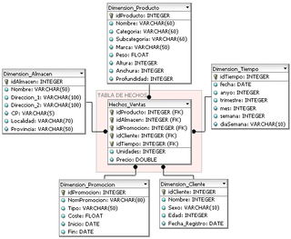
In computing, the star schema or star model is the simplest style of data mart schema and is the approach most widely used to develop data warehouses and dimensional data marts. The star schema consists of one or more fact tables referencing any number of dimension tables. The star schema is an important special case of the snowflake schema, and is more effective for handling simpler queries.
A natural key is a type of unique key in a database formed of attributes that exist and are used in the external world outside the database. In the relational model of data, a natural key is a superkey and is therefore a functional determinant for all attributes in a relation.
In data warehousing, a fact table consists of the measurements, metrics or facts of a business process. It is located at the center of a star schema or a snowflake schema surrounded by dimension tables. Where multiple fact tables are used, these are arranged as a fact constellation schema. A fact table typically has two types of columns: those that contain facts and those that are a foreign key to dimension tables. The primary key of a fact table is usually a composite key that is made up of all of its foreign keys. Fact tables contain the content of the data warehouse and store different types of measures like additive, non-additive, and semi-additive measures.
In computing, a snowflake schema or snowflake model is a logical arrangement of tables in a multidimensional database such that the entity relationship diagram resembles a snowflake shape. The snowflake schema is represented by centralized fact tables which are connected to multiple dimensions. "Snowflaking" is a method of normalizing the dimension tables in a star schema. When it is completely normalized along all the dimension tables, the resultant structure resembles a snowflake with the fact table in the middle. The principle behind snowflaking is normalization of the dimension tables by removing low cardinality attributes and forming separate tables.
A dimension is a structure that categorizes facts and measures in order to enable users to answer business questions. Commonly used dimensions are people, products, place and time.
In databases, change data capture (CDC) is a set of software design patterns used to determine and track the data that has changed so that action can be taken using the changed data. The result is a delta-driven dataset.
Data cleansing or data cleaning is the process of detecting and correcting corrupt or inaccurate records from a record set, table, or database and refers to identifying incomplete, incorrect, inaccurate or irrelevant parts of the data and then replacing, modifying, or deleting the dirty or coarse data. Data cleansing may be performed interactively with data wrangling tools, or as batch processing through scripting or a data quality firewall.
Sixth normal form (6NF) is a normal form used in relational database normalization which extends the relational algebra and generalizes relational operators to support interval data, which can be useful in temporal databases.
An entity–attribute–value model (EAV) is a data model optimized for the space-efficient storage of sparse—or ad-hoc—property or data values, intended for situations where runtime usage patterns are arbitrary, subject to user variation, or otherwise unforeseeable using a fixed design. The use-case targets applications which offer a large or rich system of defined property types, which are in turn appropriate to a wide set of entities, but where typically only a small, specific selection of these are instantiated for a given entity. Therefore, this type of data model relates to the mathematical notion of a sparse matrix. EAV is also known as object–attribute–value model, vertical database model, and open schema.
Dimensional modeling (DM) is part of the Business Dimensional Lifecycle methodology developed by Ralph Kimball which includes a set of methods, techniques and concepts for use in data warehouse design. The approach focuses on identifying the key business processes within a business and modelling and implementing these first before adding additional business processes, as a bottom-up approach. An alternative approach from Inmon advocates a top down design of the model of all the enterprise data using tools such as entity-relationship modeling (ER).
A database model is a type of data model that determines the logical structure of a database. It fundamentally determines in which manner data can be stored, organized and manipulated. The most popular example of a database model is the relational model, which uses a table-based format.
Datavault or data vault modeling is a database modeling method that is designed to provide long-term historical storage of data coming in from multiple operational systems. It is also a method of looking at historical data that deals with issues such as auditing, tracing of data, loading speed and resilience to change as well as emphasizing the need to trace where all the data in the database came from. This means that every row in a data vault must be accompanied by record source and load date attributes, enabling an auditor to trace values back to the source. The concept was published in 2000 by Dan Linstedt.
In relational databases, the log trigger or history trigger is a mechanism for automatic recording of information about changes inserting or/and updating or/and deleting rows in a database table.
The following is provided as an overview of and topical guide to databases:
References
Bruce Ottmann, Chris Angus: Data processing system, US Patent Office, Patent Number 7,003,504. February 21, 2006
Ralph Kimball:Kimball University: Handling Arbitrary Restatements of History. December 9, 2007
This page is based on this Wikipedia article Text is available under the CC BY-SA 4.0 license; additional terms may apply. Images, videos and audio are available under their respective licenses.