Econometrics is an application of statistical methods to economic data in order to give empirical content to economic relationships. More precisely, it is "the quantitative analysis of actual economic phenomena based on the concurrent development of theory and observation, related by appropriate methods of inference." An introductory economics textbook describes econometrics as allowing economists "to sift through mountains of data to extract simple relationships." Jan Tinbergen is one of the two founding fathers of econometrics. The other, Ragnar Frisch, also coined the term in the sense in which it is used today.
Causality (also called causation, or cause and effect) is an influence by which one event, process, state, or object (acause) contributes to the production of another event, process, state, or object (an effect) where the cause is partly responsible for the effect, and the effect is partly dependent on the cause. In general, a process has many causes, which are also said to be causal factors for it, and all lie in its past. An effect can in turn be a cause of, or causal factor for, many other effects, which all lie in its future. Some writers have held that causality is metaphysically prior to notions of time and space.
The phrase "correlation does not imply causation" refers to the inability to legitimately deduce a cause-and-effect relationship between two events or variables solely on the basis of an observed association or correlation between them. The idea that "correlation implies causation" is an example of a questionable-cause logical fallacy, in which two events occurring together are taken to have established a cause-and-effect relationship. This fallacy is also known by the Latin phrase cum hoc ergo propter hoc. This differs from the fallacy known as post hoc ergo propter hoc, in which an event following another is seen as a necessary consequence of the former event, and from conflation, the errant merging of two events, ideas, databases, etc., into one.
Linear trend estimation is a statistical technique that aids in the interpretation of data. When a series of measurements of a process are treated as a sequence or time series, trend estimation can be used to make and justify statements about tendencies in the data by relating the measurements to the times at which they occurred. This model can then be used to describe the behavior of the observed data.
In statistics, multicollinearity is a phenomenon in which one predictor variable in a multiple regression model can be to a large degree predicted from the others. In this situation, the coefficient estimates of the multiple regression may change erratically in response to small changes in the data or the procedure used to fit the model.
In statistics, econometrics, epidemiology and related disciplines, the method of instrumental variables (IV) is used to estimate causal relationships when controlled experiments are not feasible or when a treatment is not successfully delivered to every unit in a randomized experiment. Intuitively, IVs are used when an explanatory variable of interest is correlated with the error term (endogenous), in which case ordinary least squares and ANOVA give biased results. A valid instrument induces changes in the explanatory variable but has no independent effect on the dependent variable and is not correlated with the error term, allowing a researcher to uncover the causal effect of the explanatory variable on the dependent variable.

The Granger causality test is a statistical hypothesis test for determining whether one time series is useful in forecasting another, first proposed in 1969. Ordinarily, regressions reflect "mere" correlations, but Clive Granger argued that causality in economics could be tested for by measuring the ability to predict the future values of a time series using prior values of another time series. Since the question of "true causality" is deeply philosophical, and because of the post hoc ergo propter hoc fallacy of assuming that one thing preceding another can be used as a proof of causation, econometricians assert that the Granger test finds only "predictive causality". Using the term "causality" alone is a misnomer, as Granger-causality is better described as "precedence", or, as Granger himself later claimed in 1977, "temporally related". Rather than testing whether Xcauses Y, the Granger causality tests whether X forecastsY.
In statistics, ordinary least squares (OLS) is a type of linear least squares method for choosing the unknown parameters in a linear regression model by the principle of least squares: minimizing the sum of the squares of the differences between the observed dependent variable in the input dataset and the output of the (linear) function of the independent variable.
Cointegration is a statistical property of a collection (X1, X2, ..., Xk) of time series variables. First, all of the series must be integrated of order d (see Order of integration). Next, if a linear combination of this collection is integrated of order less than d, then the collection is said to be co-integrated. Formally, if (X,Y,Z) are each integrated of order d, and there exist coefficients a,b,c such that aX + bY + cZ is integrated of order less than d, then X, Y, and Z are cointegrated. Cointegration has become an important property in contemporary time series analysis. Time series often have trends—either deterministic or stochastic. In an influential paper, Charles Nelson and Charles Plosser (1982) provided statistical evidence that many US macroeconomic time series (like GNP, wages, employment, etc.) have stochastic trends.
This glossary of statistics and probability is a list of definitions of terms and concepts used in the mathematical sciences of statistics and probability, their sub-disciplines, and related fields. For additional related terms, see Glossary of mathematics and Glossary of experimental design.

In causal inference, a confounder is a variable that influences both the dependent variable and independent variable, causing a spurious association. Confounding is a causal concept, and as such, cannot be described in terms of correlations or associations. The existence of confounders is an important quantitative explanation why correlation does not imply causation. Some notations are explicitly designed to identify the existence, possible existence, or non-existence of confounders in causal relationships between elements of a system.
In statistics, the Durbin–Watson statistic is a test statistic used to detect the presence of autocorrelation at lag 1 in the residuals from a regression analysis. It is named after James Durbin and Geoffrey Watson. The small sample distribution of this ratio was derived by John von Neumann. Durbin and Watson applied this statistic to the residuals from least squares regressions, and developed bounds tests for the null hypothesis that the errors are serially uncorrelated against the alternative that they follow a first order autoregressive process. Note that the distribution of this test statistic does not depend on the estimated regression coefficients and the variance of the errors.

In the philosophy of science, a causal model is a conceptual model that describes the causal mechanisms of a system. Several types of causal notation may be used in the development of a causal model. Causal models can improve study designs by providing clear rules for deciding which independent variables need to be included/controlled for.

In statistics, a mediation model seeks to identify and explain the mechanism or process that underlies an observed relationship between an independent variable and a dependent variable via the inclusion of a third hypothetical variable, known as a mediator variable. Rather than a direct causal relationship between the independent variable and the dependent variable, a mediation model proposes that the independent variable influences the mediator variable, which in turn influences the dependent variable. Thus, the mediator variable serves to clarify the nature of the relationship between the independent and dependent variables.
In causal models, controlling for a variable means binning data according to measured values of the variable. This is typically done so that the variable can no longer act as a confounder in, for example, an observational study or experiment.
An error correction model (ECM) belongs to a category of multiple time series models most commonly used for data where the underlying variables have a long-run common stochastic trend, also known as cointegration. ECMs are a theoretically-driven approach useful for estimating both short-term and long-term effects of one time series on another. The term error-correction relates to the fact that last-period's deviation from a long-run equilibrium, the error, influences its short-run dynamics. Thus ECMs directly estimate the speed at which a dependent variable returns to equilibrium after a change in other variables.
Causal inference is the process of determining the independent, actual effect of a particular phenomenon that is a component of a larger system. The main difference between causal inference and inference of association is that causal inference analyzes the response of an effect variable when a cause of the effect variable is changed. The study of why things occur is called etiology, and can be described using the language of scientific causal notation. Causal inference is said to provide the evidence of causality theorized by causal reasoning.
Causal research, is the investigation of cause-relationships. To determine causality, variation in the variable presumed to influence the difference in another variable(s) must be detected, and then the variations from the other variable(s) must be calculated (s). Other confounding influences must be controlled for so they don't distort the results, either by holding them constant in the experimental creation of evidence. This type of research is very complex and the researcher can never be completely certain that there are no other factors influencing the causal relationship, especially when dealing with people's attitudes and motivations. There are often much deeper psychological considerations that even the respondent may not be aware of.
In statistics, econometrics, epidemiology, genetics and related disciplines, causal graphs are probabilistic graphical models used to encode assumptions about the data-generating process.
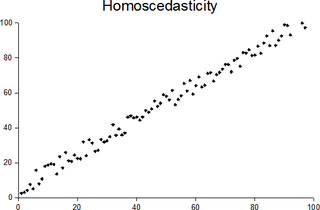
In statistics, a sequence of random variables is homoscedastic if all its random variables have the same finite variance; this is also known as homogeneity of variance. The complementary notion is called heteroscedasticity, also known as heterogeneity of variance. The spellings homoskedasticity and heteroskedasticity are also frequently used. Assuming a variable is homoscedastic when in reality it is heteroscedastic results in unbiased but inefficient point estimates and in biased estimates of standard errors, and may result in overestimating the goodness of fit as measured by the Pearson coefficient.


