
In physics and electrical engineering, a cutoff frequency, corner frequency, or break frequency is a boundary in a system's frequency response at which energy flowing through the system begins to be reduced rather than passing through.

The Navier–Stokes equations are partial differential equations which describe the motion of viscous fluid substances. They were named after French engineer and physicist Claude-Louis Navier and the Irish physicist and mathematician George Gabriel Stokes. They were developed over several decades of progressively building the theories, from 1822 (Navier) to 1842–1850 (Stokes).

In fluid dynamics, gravity waves are waves generated in a fluid medium or at the interface between two media when the force of gravity or buoyancy tries to restore equilibrium. An example of such an interface is that between the atmosphere and the ocean, which gives rise to wind waves.

In mathematics and physics, the heat equation is a certain partial differential equation. Solutions of the heat equation are sometimes known as caloric functions. The theory of the heat equation was first developed by Joseph Fourier in 1822 for the purpose of modeling how a quantity such as heat diffuses through a given region.

In physics and fluid mechanics, a boundary layer is the thin layer of fluid in the immediate vicinity of a bounding surface formed by the fluid flowing along the surface. The fluid's interaction with the wall induces a no-slip boundary condition. The flow velocity then monotonically increases above the surface until it returns to the bulk flow velocity. The thin layer consisting of fluid whose velocity has not yet returned to the bulk flow velocity is called the velocity boundary layer.

In theoretical physics, the (one-dimensional) nonlinear Schrödinger equation (NLSE) is a nonlinear variation of the Schrödinger equation. It is a classical field equation whose principal applications are to the propagation of light in nonlinear optical fibers and planar waveguides and to Bose–Einstein condensates confined to highly anisotropic, cigar-shaped traps, in the mean-field regime. Additionally, the equation appears in the studies of small-amplitude gravity waves on the surface of deep inviscid (zero-viscosity) water; the Langmuir waves in hot plasmas; the propagation of plane-diffracted wave beams in the focusing regions of the ionosphere; the propagation of Davydov's alpha-helix solitons, which are responsible for energy transport along molecular chains; and many others. More generally, the NLSE appears as one of universal equations that describe the evolution of slowly varying packets of quasi-monochromatic waves in weakly nonlinear media that have dispersion. Unlike the linear Schrödinger equation, the NLSE never describes the time evolution of a quantum state. The 1D NLSE is an example of an integrable model.
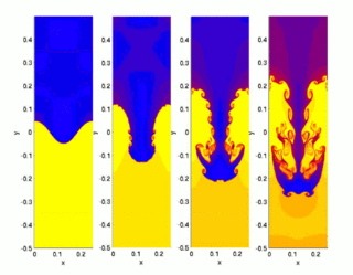
The Rayleigh–Taylor instability, or RT instability, is an instability of an interface between two fluids of different densities which occurs when the lighter fluid is pushing the heavier fluid. Examples include the behavior of water suspended above oil in the gravity of Earth, mushroom clouds like those from volcanic eruptions and atmospheric nuclear explosions, supernova explosions in which expanding core gas is accelerated into denser shell gas, instabilities in plasma fusion reactors and inertial confinement fusion.
In physics and fluid mechanics, a Blasius boundary layer describes the steady two-dimensional laminar boundary layer that forms on a semi-infinite plate which is held parallel to a constant unidirectional flow. Falkner and Skan later generalized Blasius' solution to wedge flow, i.e. flows in which the plate is not parallel to the flow.
In fluid mechanics, potential vorticity (PV) is a quantity which is proportional to the dot product of vorticity and stratification. This quantity, following a parcel of air or water, can only be changed by diabatic or frictional processes. It is a useful concept for understanding the generation of vorticity in cyclogenesis, especially along the polar front, and in analyzing flow in the ocean.
The Orr–Sommerfeld equation, in fluid dynamics, is an eigenvalue equation describing the linear two-dimensional modes of disturbance to a viscous parallel flow. The solution to the Navier–Stokes equations for a parallel, laminar flow can become unstable if certain conditions on the flow are satisfied, and the Orr–Sommerfeld equation determines precisely what the conditions for hydrodynamic stability are.
The derivation of the Navier–Stokes equations as well as its application and formulation for different families of fluids, is an important exercise in fluid dynamics with applications in mechanical engineering, physics, chemistry, heat transfer, and electrical engineering. A proof explaining the properties and bounds of the equations, such as Navier–Stokes existence and smoothness, is one of the important unsolved problems in mathematics.
Acoustic streaming is a steady flow in a fluid driven by the absorption of high amplitude acoustic oscillations. This phenomenon can be observed near sound emitters, or in the standing waves within a Kundt's tube. Acoustic streaming was explained first by Lord Rayleigh in 1884. It is the less-known opposite of sound generation by a flow.
In fluid dynamics, a Tollmien–Schlichting wave is a streamwise unstable wave which arises in a bounded shear flow. It is one of the more common methods by which a laminar bounded shear flow transitions to turbulence. The waves are initiated when some disturbance interacts with leading edge roughness in a process known as receptivity. These waves are slowly amplified as they move downstream until they may eventually grow large enough that nonlinearities take over and the flow transitions to turbulence.

In fluid dynamics, the Falkner–Skan boundary layer describes the steady two-dimensional laminar boundary layer that forms on a wedge, i.e. flows in which the plate is not parallel to the flow. It is also representative of flow on a flat plate with an imposed pressure gradient along the plate length, a situation often encountered in wind tunnel flow. It is a generalization of the flat plate Blasius boundary layer in which the pressure gradient along the plate is zero.
Skin friction drag is a type of aerodynamic or hydrodynamic drag, which is resistant force exerted on an object moving in a fluid. Skin friction drag is caused by the viscosity of fluids and is developed from laminar drag to turbulent drag as a fluid moves on the surface of an object. Skin friction drag is generally expressed in terms of the Reynolds number, which is the ratio between inertial force and viscous force.
In fluid dynamics, Stokes problem also known as Stokes second problem or sometimes referred to as Stokes boundary layer or Oscillating boundary layer is a problem of determining the flow created by an oscillating solid surface, named after Sir George Stokes. This is considered one of the simplest unsteady problems that has an exact solution for the Navier-Stokes equations. In turbulent flow, this is still named a Stokes boundary layer, but now one has to rely on experiments, numerical simulations or approximate methods in order to obtain useful information on the flow.
In fluid dynamics, Beltrami flows are flows in which the vorticity vector and the velocity vector are parallel to each other. In other words, Beltrami flow is a flow where Lamb vector is zero. It is named after the Italian mathematician Eugenio Beltrami due to his derivation of the Beltrami vector field, while initial developments in fluid dynamics were done by the Russian scientist Ippolit S. Gromeka in 1881.
In fluid dynamics, Kerr–Dold vortex is an exact solution of Navier–Stokes equations, which represents steady periodic vortices superposed on the stagnation point flow. The solution was discovered by Oliver S. Kerr and John W. Dold in 1994. These steady solutions exist as a result of a balance between vortex stretching by the extensional flow and viscous dissipation, which are similar to Burgers vortex. These vortices were observed experimentally in a four-roll mill apparatus by Lagnado and L. Gary Leal.
Schneider flow describes the axisymmetric outer flow induced by a laminar or turbulent jet having a large jet Reynolds number or by a laminar plume with a large Grashof number, in the case where the fluid domain is bounded by a wall. When the jet Reynolds number or the plume Grashof number is large, the full flow field constitutes two regions of different extent: a thin boundary-layer flow that may identified as the jet or as the plume and a slowly moving fluid in the large outer region encompassing the jet or the plume. The Schneider flow describing the latter motion is an exact solution of the Navier-Stokes equations, discovered by Wilhelm Schneider in 1981. The solution was discovered also by A. A. Golubinskii and V. V. Sychev in 1979, however, was never applied to flows entrained by jets. The solution is an extension of Taylor's potential flow solution to arbitrary Reynolds number.

The Rayleigh–Kuo criterion is a stability condition for a fluid. This criterion determines whether or not a barotropic instability can occur, leading to the presence of vortices. The Kuo criterion states that for barotropic instability to occur, the gradient of the absolute vorticity must change its sign at some point within the boundaries of the current. Note that this criterion is a necessary condition, so if it does not hold it is not possible for a barotropic instability to form. But it is not a sufficient condition, meaning that if the criterion is met, this does not automatically mean that the fluid is unstable. If the criterion is not met, it is certain that the flow is stable.


