Backjumping

In backtracking algorithms, backjumping is a technique that reduces search space, therefore increasing efficiency. While backtracking always goes up one level in the search tree when all values for a variable have been tested, backjumping may go up more levels. In this article, a fixed order of evaluation of variables ${\displaystyle x_{1},\ldots ,x_{n}}$ is used, but the same considerations apply to a dynamic order of evaluation.

• 
  A search tree visited by regular backtracking
• 
  A backjump: the grey node is not visited

Definition

Whenever backtracking has tried all values for a variable without finding any solution, it reconsiders the last of the previously assigned variables, changing its value or further backtracking if no other values are to be tried. If ${\displaystyle x_{1}=a_{1},\ldots ,x_{k}=a_{k}}$ is the current partial assignment and all values for ${\displaystyle x_{k+1}}$ have been tried without finding a solution, backtracking concludes that no solution extending ${\displaystyle x_{1}=a_{1},\ldots ,x_{k}=a_{k}}$ exists. The algorithm then "goes up" to ${\displaystyle x_{k}}$, changing ${\displaystyle x_{k}}$'s value if possible, backtracking again otherwise.

The partial assignment is not always necessary in full to prove that no value of ${\displaystyle x_{k+1}}$ leads to a solution. In particular, a prefix of the partial assignment may have the same property, that is, there exists an index ${\displaystyle j<k}$ such that ${\displaystyle x_{1},\ldots ,x_{j}=a_{1},\ldots ,a_{j}}$ cannot be extended to form a solution with whatever value for ${\displaystyle x_{k+1}}$. If the algorithm can prove this fact, it can directly consider a different value for ${\displaystyle x_{j}}$ instead of reconsidering ${\displaystyle x_{k}}$ as it would normally do.

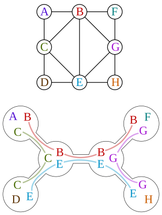
An example in which the current assignment to ${\displaystyle x_{1}x_{2}x_{3}x_{4}}$ has been unsuccessfully tried with every possible value of ${\displaystyle x_{5}}$. Backtracking goes back to ${\displaystyle x_{4}}$, trying to assign it a new value.	Instead of backtracking, the algorithm makes some further elaboration, proving that the evaluations ${\displaystyle x_{1}x_{2}x_{5}=211}$, ${\displaystyle x_{1}x_{2}x_{5}=212}$, and ${\displaystyle x_{1}x_{2}x_{5}=213}$ are not part of any solution.	As a result, the current evaluation of ${\displaystyle x_{1}x_{2}}$ is not part of any solution, and the algorithm can directly backjump to ${\displaystyle x_{2}}$, trying a new value for it.

The efficiency of a backjumping algorithm depends on how high it is able to backjump. Ideally, the algorithm could jump from ${\displaystyle x_{k+1}}$ to whichever variable ${\displaystyle x_{j}}$ is such that the current assignment to ${\displaystyle x_{1},\ldots ,x_{j}}$ cannot be extended to form a solution with any value of ${\displaystyle x_{k+1}}$. If this is the case, ${\displaystyle j}$ is called a safe jump.

Establishing whether a jump is safe is not always feasible, as safe jumps are defined in terms of the set of solutions, which is what the algorithm is trying to find. In practice, backjumping algorithms use the lowest index they can efficiently prove to be a safe jump. Different algorithms use different methods for determining whether a jump is safe. These methods have different cost, but a higher cost of finding a higher safe jump may be traded off a reduced amount of search due to skipping parts of the search tree.

Backjumping at leaf nodes

The simplest condition in which backjumping is possible is when all values of a variable have been proved inconsistent without further branching. In constraint satisfaction, a partial evaluation is consistent if and only if it satisfies all constraints involving the assigned variables, and inconsistent otherwise. It might be the case that a consistent partial solution cannot be extended to a consistent complete solution because some of the unassigned variables may not be assigned without violating other constraints.

The condition in which all values of a given variable ${\displaystyle x_{k+1}}$ are inconsistent with the current partial solution ${\displaystyle x_{1},\ldots ,x_{k}=a_{1},\ldots ,a_{k}}$ is called a leaf dead end. This happens exactly when the variable ${\displaystyle x_{k+1}}$ is a leaf of the search tree (which correspond to nodes having only leaves as children in the figures of this article.)

The backjumping algorithm by John Gaschnig does a backjump only in leaf dead ends. In other words, it works differently from backtracking only when every possible value of ${\displaystyle x_{k+1}}$ has been tested and resulted inconsistent without the need of branching over another variable.

A safe jump can be found by simply evaluating, for every value ${\displaystyle a_{k+1}}$, the shortest prefix of ${\displaystyle x_{1},\ldots ,x_{k}=a_{1},\ldots ,a_{k}}$ inconsistent with ${\displaystyle x_{k+1}=a_{k+1}}$. In other words, if ${\displaystyle a_{k+1}}$ is a possible value for ${\displaystyle x_{k+1}}$, the algorithm checks the consistency of the following evaluations:

${\displaystyle x_{1}=a_{1}}$	...	${\displaystyle x_{k-1}=a_{k-1}}$	${\displaystyle x_{k}=a_{k}}$	${\displaystyle x_{k+1}=a_{k+1}}$
${\displaystyle x_{1}=a_{1}}$	...	${\displaystyle x_{k-1}=a_{k-1}}$		${\displaystyle x_{k+1}=a_{k+1}}$
...
${\displaystyle x_{1}=a_{1}}$				${\displaystyle x_{k+1}=a_{k+1}}$

The smallest index (lowest the listing) for which evaluations are inconsistent would be a safe jump if ${\displaystyle x_{k+1}=a_{k+1}}$ were the only possible value for ${\displaystyle x_{k+1}}$. Since every variable can usually take more than one value, the maximal index that comes out from the check for each value is a safe jump, and is the point where John Gaschnig's algorithm jumps.

In practice, the algorithm can check the evaluations above at the same time it is checking the consistency of ${\displaystyle x_{k+1}=a_{k+1}}$.

Backjumping at internal nodes

The previous algorithm only backjumps when the values of a variable can be shown inconsistent with the current partial solution without further branching. In other words, it allows for a backjump only at leaf nodes in the search tree.

An internal node of the search tree represents an assignment of a variable that is consistent with the previous ones. If no solution extends this assignment, the previous algorithm always backtracks: no backjump is done in this case.

Backjumping at internal nodes cannot be done as for leaf nodes. Indeed, if some evaluations of ${\displaystyle x_{k+1}}$ required branching, it is because they are consistent with the current assignment. As a result, searching for a prefix that is inconsistent with these values of the last variable does not succeed.

In such cases, what proved an evaluation ${\displaystyle x_{k+1}=a_{k+1}}$ not to be part of a solution with the current partial evaluation ${\displaystyle x_{1},\ldots ,x_{k}}$ is the recursive search. In particular, the algorithm "knows" that no solution exists from this point on because it comes back to this node instead of stopping after having found a solution.

This return is due to a number of dead ends, points where the algorithm has proved a partial solution inconsistent. In order to further backjump, the algorithm has to take into account that the impossibility of finding solutions is due to these dead ends. In particular, the safe jumps are indexes of prefixes that still make these dead ends to be inconsistent partial solutions.

In this example, the algorithm come back to ${\displaystyle x_{k+1}}$, after trying all its possible values, because of the three crossed points of inconsistency.	The second point remains inconsistent even if the values of ${\displaystyle x_{k+1}}$ and ${\displaystyle x_{k}}$ are removed from its partial evaluation (note that the values of a variable are in its children)	The other inconsistent evaluations remains so even without ${\displaystyle x_{k-2}}$, ${\displaystyle x_{k-1}}$, and ${\displaystyle x_{k}}$	The algorithm can backjump to ${\displaystyle x_{k-2}}$ since this is the lowest variables that maintains all inconsistencies. A new value for ${\displaystyle x_{k-2}}$ will be tried.

In other words, when all values of ${\displaystyle x_{k+1}}$ have been tried, the algorithm can backjump to a previous variable ${\displaystyle x_{i}}$ provided that the current truth evaluation of ${\displaystyle x_{1},\ldots ,x_{i}}$ is inconsistent with all the truth evaluations of ${\displaystyle x_{k+1},x_{k+2},...}$ in the leaf nodes that are descendants of the node ${\displaystyle x_{k+1}}$.

Simplifications

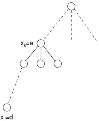
While looking for a possible backjump for ${\displaystyle x_{k+1}}$ or one its ancestors, all nodes in the shaded area can be ignored.

Due to the potentially high number of nodes that are in the subtree of ${\displaystyle x_{k+1}}$, the information that is necessary to safely backjump from ${\displaystyle x_{k+1}}$ is collected during the visit of its subtree. Finding a safe jump can be simplified by two considerations. The first is that the algorithm needs a safe jump, but still works with a jump that is not the highest possible safe jump.

The second simplification is that nodes in the subtree of ${\displaystyle x_{l}}$ that have been skipped by a backjump can be ignored while looking for a backjump for ${\displaystyle x_{l}}$. More precisely, all nodes skipped by a backjump from node ${\displaystyle x_{m}}$ up to node ${\displaystyle x_{l}}$ are irrelevant to the subtree rooted at ${\displaystyle x_{m}}$, and also irrelevant are their other subtrees.

Indeed, if an algorithm went down from node ${\displaystyle x_{l}}$ to ${\displaystyle x_{m}}$ via a path but backjumps in its way back, then it could have gone directly from ${\displaystyle x_{l}}$ to ${\displaystyle x_{m}}$ instead. Indeed, the backjump indicates that the nodes between ${\displaystyle x_{l}}$ and ${\displaystyle x_{m}}$ are irrelevant to the subtree rooted at ${\displaystyle x_{m}}$. In other words, a backjump indicates that the visit of a region of the search tree had been a mistake. This part of the search tree can therefore be ignored when considering a possible backjump from ${\displaystyle x_{l}}$ or from one of its ancestors.

Variables whose values are sufficient to prove unsatisfiability in the subtree rooted at a node are collected in the node and sent (after removing the variable of the node) to the node above when retracting.

This fact can be exploited by collecting, in each node, a set of previously assigned variables whose evaluation suffices to prove that no solution exists in the subtree rooted at the node. This set is built during the execution of the algorithm. When retracting from a node, this set is removed the variable of the node and collected in the set of the destination of backtracking or backjumping. Since nodes that are skipped from backjumping are never retracted from, their sets are automatically ignored.

Graph-based backjumping

The rationale of graph-based backjumping is that a safe jump can be found by checking which of the variables ${\displaystyle x_{1},\ldots ,x_{k}}$ are in a constraint with the variables ${\displaystyle x_{k+1},x_{k+2},...}$ that are instantiated in leaf nodes. For every leaf node and every variable ${\displaystyle x_{i}}$ of index ${\displaystyle i>k}$ that is instantiated there, the indexes less than or equal to ${\displaystyle k}$ whose variable is in a constraint with ${\displaystyle x_{i}}$ can be used to find safe jumps. In particular, when all values for ${\displaystyle x_{k+1}}$ have been tried, this set contains the indexes of the variables whose evaluations allow proving that no solution can be found by visiting the subtree rooted at ${\displaystyle x_{k+1}}$. As a result, the algorithm can backjump to the highest index in this set.

The fact that nodes skipped by backjumping can be ignored when considering a further backjump can be exploited by the following algorithm. When retracting from a leaf node, the set of variables that are in constraint with it is created and "sent back" to its parent, or ancestor in case of backjumping. At every internal node, a set of variables is maintained. Every time a set of variables is received from one of its children or descendant, their variables are added to the maintained set. When further backtracking or backjumping from the node, the variable of the node is removed from this set, and the set is sent to the node that is the destination of backtracking or backjumping. This algorithm works because the set maintained in a node collects all variables that are relevant to prove unsatisfiability in the leaves that are descendant of this node. Since sets of variables are only sent when retracing from nodes, the sets collected at nodes skipped by backjumping are automatically ignored.

Conflict-based backjumping (aka conflict-directed backjumping (cbj))

A still more refined backjumping algorithm, sometimes able to achieve larger backjumps, is based on checking not only the common presence of two variables in the same constraint but also on whether the constraint actually caused inconsistency. In particular, this algorithm collects one of the violated constraints in every leaf. At every node, the highest index of a variable that is in one of the constraints collected at the leaves is a safe jump.

While the violated constraint chosen in each leaf does not affect the safeness of the resulting jump, choosing constraints of highest possible indices increases the highness of the jump. For this reason, conflict-based backjumping orders constraints in such a way constraints over lower indices variables are preferred over constraints on higher index variables.

Formally, a constraint ${\displaystyle C}$ is preferred over another one ${\displaystyle D}$ if the highest index of a variable in ${\displaystyle C}$ but not in ${\displaystyle D}$ is lower than the highest index of a variable in ${\displaystyle D}$ but not in ${\displaystyle C}$. In other words, excluding common variables, the constraint that has the all lower indices is preferred.

In a leaf node, the algorithm chooses the lowest index ${\displaystyle i}$ such that ${\displaystyle x_{1},\ldots ,x_{i}}$ is inconsistent with the last variable evaluated in the leaf. Among the constraints that are violated in this evaluation, it chooses the most preferred one, and collects all its indices less than ${\displaystyle k+1}$. This way, when the algorithm comes back to the variable ${\displaystyle x_{k+1}}$, the lowest collected index identifies a safe jump.

In practice, this algorithm is simplified by collecting all indices in a single set, instead of creating a set for every value of ${\displaystyle k}$. In particular, the algorithm collects, in each node, all sets coming from its descendants that have not been skipped by backjumping. When retracting from this node, this set is removed the variable of the node and collected into the destination of backtracking or backjumping.

Conflict-directed backjumping was proposed for Constraint Satisfaction Problems by Patrick Prosser in his seminal 1993 paper.

See also

• Backtracking
• Constraint learning

References

• Dechter, Rina (2003). Constraint Processing . Morgan Kaufmann. ISBN   1-55860-890-7.
• Prosser, Patrick (1993). "Hybrid Algorithms for the Constraint Satisfaction Problem" (PDF). Computational Intelligence 9(3).