
In physics, the Navier–Stokes equations are certain partial differential equations which describe the motion of viscous fluid substances, named after French engineer and physicist Claude-Louis Navier and Anglo-Irish physicist and mathematician George Gabriel Stokes. They were developed over several decades of progressively building the theories, from 1822 (Navier) to 1842–1850 (Stokes).
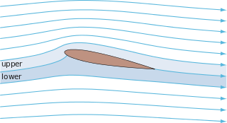
In fluid dynamics, potential flow describes the velocity field as the gradient of a scalar function: the velocity potential. As a result, a potential flow is characterized by an irrotational velocity field, which is a valid approximation for several applications. The irrotationality of a potential flow is due to the curl of the gradient of a scalar always being equal to zero.
In 1851, George Gabriel Stokes derived an expression, now known as Stokes law, for the frictional force – also called drag force – exerted on spherical objects with very small Reynolds numbers in a viscous fluid. Stokes' law is derived by solving the Stokes flow limit for small Reynolds numbers of the Navier–Stokes equations.
In fluid dynamics, Couette flow is the flow of a viscous fluid in the space between two surfaces, one of which is moving tangentially relative to the other. The relative motion of the surfaces imposes a shear stress on the fluid and induces flow. Depending on the definition of the term, there may also be an applied pressure gradient in the flow direction.
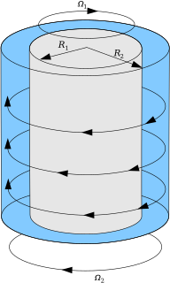
In fluid dynamics, the Taylor–Couette flow consists of a viscous fluid confined in the gap between two rotating cylinders. For low angular velocities, measured by the Reynolds number Re, the flow is steady and purely azimuthal. This basic state is known as circular Couette flow, after Maurice Marie Alfred Couette, who used this experimental device as a means to measure viscosity. Sir Geoffrey Ingram Taylor investigated the stability of Couette flow in a ground-breaking paper. Taylor's paper became a cornerstone in the development of hydrodynamic stability theory and demonstrated that the no-slip condition, which was in dispute by the scientific community at the time, was the correct boundary condition for viscous flows at a solid boundary.

In fluid dynamics, the Lamb–Oseen vortex models a line vortex that decays due to viscosity. This vortex is named after Horace Lamb and Carl Wilhelm Oseen.
Hill's spherical vortex is an exact solution of the Euler equations that is commonly used to model a vortex ring. The solution is also used to model the velocity distribution inside a spherical drop of one fluid moving at a constant velocity through another fluid at small Reynolds number. The vortex is named after Micaiah John Muller Hill who discovered the exact solution in 1894. The two-dimensional analogue of this vortex is the Lamb–Chaplygin dipole.

In fluid dynamics, Görtler vortices are secondary flows that appear in a boundary layer flow along a concave wall. If the boundary layer is thin compared to the radius of curvature of the wall, the pressure remains constant across the boundary layer. On the other hand, if the boundary layer thickness is comparable to the radius of curvature, the centrifugal action creates a pressure variation across the boundary layer. This leads to the centrifugal instability of the boundary layer and consequent formation of Görtler vortices.

In fluid dynamics, the Stokes stream function is used to describe the streamlines and flow velocity in a three-dimensional incompressible flow with axisymmetry. A surface with a constant value of the Stokes stream function encloses a streamtube, everywhere tangential to the flow velocity vectors. Further, the volume flux within this streamtube is constant, and all the streamlines of the flow are located on this surface. The velocity field associated with the Stokes stream function is solenoidal—it has zero divergence. This stream function is named in honor of George Gabriel Stokes.
Bending of plates, or plate bending, refers to the deflection of a plate perpendicular to the plane of the plate under the action of external forces and moments. The amount of deflection can be determined by solving the differential equations of an appropriate plate theory. The stresses in the plate can be calculated from these deflections. Once the stresses are known, failure theories can be used to determine whether a plate will fail under a given load.
A vortex sheet is a term used in fluid mechanics for a surface across which there is a discontinuity in fluid velocity, such as in slippage of one layer of fluid over another. While the tangential components of the flow velocity are discontinuous across the vortex sheet, the normal component of the flow velocity is continuous. The discontinuity in the tangential velocity means the flow has infinite vorticity on a vortex sheet.
Blade element momentum theory is a theory that combines both blade element theory and momentum theory. It is used to calculate the local forces on a propeller or wind-turbine blade. Blade element theory is combined with momentum theory to alleviate some of the difficulties in calculating the induced velocities at the rotor.
In fluid dynamics, the Burgers vortex or Burgers–Rott vortex is an exact solution to the Navier–Stokes equations governing viscous flow, named after Jan Burgers and Nicholas Rott. The Burgers vortex describes a stationary, self-similar flow. An inward, radial flow, tends to concentrate vorticity in a narrow column around the symmetry axis. At the same time, viscous diffusion tends to spread the vorticity. The stationary Burgers vortex arises when the two effects balance.
Skin friction drag is a type of aerodynamic drag, which is resistant force exerted on an object moving in a fluid. Skin friction drag is caused by the viscosity of fluids and is developed from laminar drag to turbulent drag as a fluid moves on the surface of an object. Skin friction drag is generally expressed in terms of the Reynolds number, which is the ratio between inertial force and viscous force.
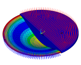
Von Kármán swirling flow is a flow created by a uniformly rotating infinitely long plane disk, named after Theodore von Kármán who solved the problem in 1921. The rotating disk acts as a fluid pump and is used as a model for centrifugal fans or compressors. This flow is classified under the category of steady flows in which vorticity generated at a solid surface is prevented from diffusing far away by an opposing convection, the other examples being the Blasius boundary layer with suction, stagnation point flow etc.
In fluid dynamics Jeffery–Hamel flow is a flow created by a converging or diverging channel with a source or sink of fluid volume at the point of intersection of the two plane walls. It is named after George Barker Jeffery(1915) and Georg Hamel(1917), but it has subsequently been studied by many major scientists such as von Kármán and Levi-Civita, Walter Tollmien, F. Noether, W.R. Dean, Rosenhead, Landau, G.K. Batchelor etc. A complete set of solutions was described by Edward Fraenkel in 1962.
In fluid dynamics, stagnation point flow represents the flow of a fluid in the immediate neighborhood of a stagnation point with which the stagnation point is identified for a potential flow or inviscid flow. The flow specifically considers a class of stagnation points known as saddle points where the incoming streamlines gets deflected and directed outwards in a different direction; the streamline deflections are guided by separatrices. The flow in the neighborhood of the stagnation point or line can generally be described using potential flow theory, although viscous effects cannot be neglected if the stagnation point lies on a solid surface.
In fluid dynamics, Rayleigh problem also known as Stokes first problem is a problem of determining the flow created by a sudden movement of an infinitely long plate from rest, named after Lord Rayleigh and Sir George Stokes. This is considered as one of the simplest unsteady problem that have exact solution for the Navier-Stokes equations. The impulse movement of semi-infinite plate was studied by Keith Stewartson.

In fluid dynamics, Stokes problem also known as Stokes second problem or sometimes referred to as Stokes boundary layer or Oscillating boundary layer is a problem of determining the flow created by an oscillating solid surface, named after Sir George Stokes. This is considered one of the simplest unsteady problem that have exact solution for the Navier-Stokes equations. In turbulent flow, this is still named a Stokes boundary layer, but now one has to rely on experiments, numerical simulations or approximate methods in order to obtain useful information on the flow.
In fluid dynamics, Hicks equation or sometimes also referred as Bragg–Hawthorne equation or Squire–Long equation is a partial differential equation that describes the distribution of stream function for axisymmetric inviscid fluid, named after William Mitchinson Hicks, who derived it first in 1898. The equation was also re-derived by Stephen Bragg and William Hawthorne in 1950 and by Robert R. Long in 1953 and by Herbert Squire in 1956. The Hicks equation without swirl was first introduced by George Gabriel Stokes in 1842. The Grad–Shafranov equation appearing in plasma physics also takes the same form as the Hicks equation.


