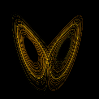
In mathematics, a dynamical system is a system in which a function describes the time dependence of a point in an ambient space, such as in a parametric curve. Examples include the mathematical models that describe the swinging of a clock pendulum, the flow of water in a pipe, the random motion of particles in the air, and the number of fish each springtime in a lake. The most general definition unifies several concepts in mathematics such as ordinary differential equations and ergodic theory by allowing different choices of the space and how time is measured. Time can be measured by integers, by real or complex numbers or can be a more general algebraic object, losing the memory of its physical origin, and the space may be a manifold or simply a set, without the need of a smooth space-time structure defined on it.

In mathematics, an integral is the continuous analog of a sum, which is used to calculate areas, volumes, and their generalizations. Integration, the process of computing an integral, is one of the two fundamental operations of calculus, the other being differentiation. Integration was initially used to solve problems in mathematics and physics, such as finding the area under a curve, or determining displacement from velocity. Usage of integration expanded to a wide variety of scientific fields thereafter.
Numerical analysis is the study of algorithms that use numerical approximation for the problems of mathematical analysis. It is the study of numerical methods that attempt to find approximate solutions of problems rather than the exact ones. Numerical analysis finds application in all fields of engineering and the physical sciences, and in the 21st century also the life and social sciences like economics, medicine, business and even the arts. Current growth in computing power has enabled the use of more complex numerical analysis, providing detailed and realistic mathematical models in science and engineering. Examples of numerical analysis include: ordinary differential equations as found in celestial mechanics, numerical linear algebra in data analysis, and stochastic differential equations and Markov chains for simulating living cells in medicine and biology.

In mathematics, a partial differential equation (PDE) is an equation which involves a multivariable function and one or more of its partial derivatives.

In mathematics, the Lyapunov exponent or Lyapunov characteristic exponent of a dynamical system is a quantity that characterizes the rate of separation of infinitesimally close trajectories. Quantitatively, two trajectories in phase space with initial separation vector diverge at a rate given by

In analysis, numerical integration comprises a broad family of algorithms for calculating the numerical value of a definite integral. The term numerical quadrature is more or less a synonym for "numerical integration", especially as applied to one-dimensional integrals. Some authors refer to numerical integration over more than one dimension as cubature; others take "quadrature" to include higher-dimensional integration.
Pseudo-spectral methods, also known as discrete variable representation (DVR) methods, are a class of numerical methods used in applied mathematics and scientific computing for the solution of partial differential equations. They are closely related to spectral methods, but complement the basis by an additional pseudo-spectral basis, which allows representation of functions on a quadrature grid. This simplifies the evaluation of certain operators, and can considerably speed up the calculation when using fast algorithms such as the fast Fourier transform.
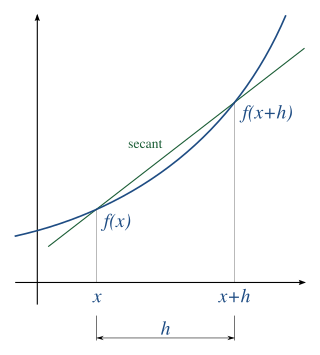
In numerical analysis, numerical differentiation algorithms estimate the derivative of a mathematical function or function subroutine using values of the function and perhaps other knowledge about the function.
In mathematics, a differential equation is an equation that relates one or more unknown functions and their derivatives. In applications, the functions generally represent physical quantities, the derivatives represent their rates of change, and the differential equation defines a relationship between the two. Such relations are common; therefore, differential equations play a prominent role in many disciplines including engineering, physics, economics, and biology.
Numerical methods for partial differential equations is the branch of numerical analysis that studies the numerical solution of partial differential equations (PDEs).
In mathematics, a differential-algebraic system of equations (DAE) is a system of equations that either contains differential equations and algebraic equations, or is equivalent to such a system.

In statistics, kernel density estimation (KDE) is the application of kernel smoothing for probability density estimation, i.e., a non-parametric method to estimate the probability density function of a random variable based on kernels as weights. KDE answers a fundamental data smoothing problem where inferences about the population are made based on a finite data sample. In some fields such as signal processing and econometrics it is also termed the Parzen–Rosenblatt window method, after Emanuel Parzen and Murray Rosenblatt, who are usually credited with independently creating it in its current form. One of the famous applications of kernel density estimation is in estimating the class-conditional marginal densities of data when using a naive Bayes classifier, which can improve its prediction accuracy.
In mathematics a radial basis function (RBF) is a real-valued function whose value depends only on the distance between the input and some fixed point, either the origin, so that , or some other fixed point , called a center, so that . Any function that satisfies the property is a radial function. The distance is usually Euclidean distance, although other metrics are sometimes used. They are often used as a collection which forms a basis for some function space of interest, hence the name.
Lloyd Nicholas Trefethen is an American mathematician, professor of numerical analysis and until 2023 head of the Numerical Analysis Group at the Mathematical Institute, University of Oxford.
Numerical linear algebra, sometimes called applied linear algebra, is the study of how matrix operations can be used to create computer algorithms which efficiently and accurately provide approximate answers to questions in continuous mathematics. It is a subfield of numerical analysis, and a type of linear algebra. Computers use floating-point arithmetic and cannot exactly represent irrational data, so when a computer algorithm is applied to a matrix of data, it can sometimes increase the difference between a number stored in the computer and the true number that it is an approximation of. Numerical linear algebra uses properties of vectors and matrices to develop computer algorithms that minimize the error introduced by the computer, and is also concerned with ensuring that the algorithm is as efficient as possible.
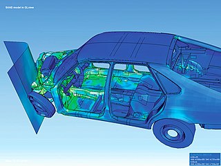
Finite element method (FEM) is a popular method for numerically solving differential equations arising in engineering and mathematical modeling. Typical problem areas of interest include the traditional fields of structural analysis, heat transfer, fluid flow, mass transport, and electromagnetic potential. Computers are usually used to perform the calculations required. With high-speed supercomputers, better solutions can be achieved and are often required to solve the largest and most complex problems.
In mathematics, the tensor product (TP) model transformation was proposed by Baranyi and Yam as key concept for higher-order singular value decomposition of functions. It transforms a function into TP function form if such a transformation is possible. If an exact transformation is not possible, then the method determines a TP function that is an approximation of the given function. Hence, the TP model transformation can provide a trade-off between approximation accuracy and complexity.

In mathematics, an ordinary differential equation (ODE) is a differential equation (DE) dependent on only a single independent variable. As with other DE, its unknown(s) consists of one function(s) and involves the derivatives of those functions. The term "ordinary" is used in contrast with partial differential equations (PDEs) which may be with respect to more than one independent variable, and, less commonly, in contrast with stochastic differential equations (SDEs) where the progression is random.
Probabilistic numerics is an active field of study at the intersection of applied mathematics, statistics, and machine learning centering on the concept of uncertainty in computation. In probabilistic numerics, tasks in numerical analysis such as finding numerical solutions for integration, linear algebra, optimization and simulation and differential equations are seen as problems of statistical, probabilistic, or Bayesian inference.

