In probability theory and statistics, the exponential distribution or negative exponential distribution is the probability distribution of the distance between events in a Poisson point process, i.e., a process in which events occur continuously and independently at a constant average rate; the distance parameter could be any meaningful mono-dimensional measure of the process, such as time between production errors, or length along a roll of fabric in the weaving manufacturing process. It is a particular case of the gamma distribution. It is the continuous analogue of the geometric distribution, and it has the key property of being memoryless. In addition to being used for the analysis of Poisson point processes it is found in various other contexts.
The primitive equations are a set of nonlinear partial differential equations that are used to approximate global atmospheric flow and are used in most atmospheric models. They consist of three main sets of balance equations:
- A continuity equation: Representing the conservation of mass.
- Conservation of momentum: Consisting of a form of the Navier–Stokes equations that describe hydrodynamical flow on the surface of a sphere under the assumption that vertical motion is much smaller than horizontal motion (hydrostasis) and that the fluid layer depth is small compared to the radius of the sphere
- A thermal energy equation: Relating the overall temperature of the system to heat sources and sinks

In theoretical physics, the (one-dimensional) nonlinear Schrödinger equation (NLSE) is a nonlinear variation of the Schrödinger equation. It is a classical field equation whose principal applications are to the propagation of light in nonlinear optical fibers and planar waveguides and to Bose–Einstein condensates confined to highly anisotropic, cigar-shaped traps, in the mean-field regime. Additionally, the equation appears in the studies of small-amplitude gravity waves on the surface of deep inviscid (zero-viscosity) water; the Langmuir waves in hot plasmas; the propagation of plane-diffracted wave beams in the focusing regions of the ionosphere; the propagation of Davydov's alpha-helix solitons, which are responsible for energy transport along molecular chains; and many others. More generally, the NLSE appears as one of universal equations that describe the evolution of slowly varying packets of quasi-monochromatic waves in weakly nonlinear media that have dispersion. Unlike the linear Schrödinger equation, the NLSE never describes the time evolution of a quantum state. The 1D NLSE is an example of an integrable model.
In fluid mechanics, potential vorticity (PV) is a quantity which is proportional to the dot product of vorticity and stratification. This quantity, following a parcel of air or water, can only be changed by diabatic or frictional processes. It is a useful concept for understanding the generation of vorticity in cyclogenesis, especially along the polar front, and in analyzing flow in the ocean.
In mathematics, the Jack function is a generalization of the Jack polynomial, introduced by Henry Jack. The Jack polynomial is a homogeneous, symmetric polynomial which generalizes the Schur and zonal polynomials, and is in turn generalized by the Heckman–Opdam polynomials and Macdonald polynomials.
Atmospheric tides are global-scale periodic oscillations of the atmosphere. In many ways they are analogous to ocean tides. Atmospheric tides can be excited by:
The omega equation is a culminating result in synoptic-scale meteorology. It is an elliptic partial differential equation, named because its left-hand side produces an estimate of vertical velocity, customarily expressed by symbol , in a pressure coordinate measuring height the atmosphere. Mathematically, , where represents a material derivative. The underlying concept is more general, however, and can also be applied to the Boussinesq fluid equation system where vertical velocity is in altitude coordinate z.

In probability theory and statistics, the Conway–Maxwell–Poisson distribution is a discrete probability distribution named after Richard W. Conway, William L. Maxwell, and Siméon Denis Poisson that generalizes the Poisson distribution by adding a parameter to model overdispersion and underdispersion. It is a member of the exponential family, has the Poisson distribution and geometric distribution as special cases and the Bernoulli distribution as a limiting case.

A two-dimensional elastic membrane under tension can support transverse vibrations. The properties of an idealized drumhead can be modeled by the vibrations of a circular membrane of uniform thickness, attached to a rigid frame. Due to the phenomenon of resonance, at certain vibration frequencies, its resonant frequencies, the membrane can store vibrational energy, the surface moving in a characteristic pattern of standing waves. This is called a normal mode. A membrane has an infinite number of these normal modes, starting with a lowest frequency one called the fundamental mode.
In fluid dynamics, Airy wave theory gives a linearised description of the propagation of gravity waves on the surface of a homogeneous fluid layer. The theory assumes that the fluid layer has a uniform mean depth, and that the fluid flow is inviscid, incompressible and irrotational. This theory was first published, in correct form, by George Biddell Airy in the 19th century.
Equatorial waves are oceanic and atmospheric waves trapped close to the equator, meaning that they decay rapidly away from the equator, but can propagate in the longitudinal and vertical directions. Wave trapping is the result of the Earth's rotation and its spherical shape which combine to cause the magnitude of the Coriolis force to increase rapidly away from the equator. Equatorial waves are present in both the tropical atmosphere and ocean and play an important role in the evolution of many climate phenomena such as El Niño. Many physical processes may excite equatorial waves including, in the case of the atmosphere, diabatic heat release associated with cloud formation, and in the case of the ocean, anomalous changes in the strength or direction of the trade winds.
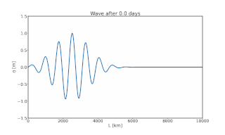
Equatorial Rossby waves, often called planetary waves, are very long, low frequency water waves found near the equator and are derived using the equatorial beta plane approximation.
In mathematics, the slow manifold of an equilibrium point of a dynamical system occurs as the most common example of a center manifold. One of the main methods of simplifying dynamical systems, is to reduce the dimension of the system to that of the slow manifold—center manifold theory rigorously justifies the modelling. For example, some global and regional models of the atmosphere or oceans resolve the so-called quasi-geostrophic flow dynamics on the slow manifold of the atmosphere/oceanic dynamics, and is thus crucial to forecasting with a climate model.
Q-vectors are used in atmospheric dynamics to understand physical processes such as vertical motion and frontogenesis. Q-vectors are not physical quantities that can be measured in the atmosphere but are derived from the quasi-geostrophic equations and can be used in the previous diagnostic situations. On meteorological charts, Q-vectors point toward upward motion and away from downward motion. Q-vectors are an alternative to the omega equation for diagnosing vertical motion in the quasi-geostrophic equations.
While geostrophic motion refers to the wind that would result from an exact balance between the Coriolis force and horizontal pressure-gradient forces, quasi-geostrophic (QG) motion refers to flows where the Coriolis force and pressure gradient forces are almost in balance, but with inertia also having an effect.

In fluid dynamics, a trochoidal wave or Gerstner wave is an exact solution of the Euler equations for periodic surface gravity waves. It describes a progressive wave of permanent form on the surface of an incompressible fluid of infinite depth. The free surface of this wave solution is an inverted (upside-down) trochoid – with sharper crests and flat troughs. This wave solution was discovered by Gerstner in 1802, and rediscovered independently by Rankine in 1863.

Conditional symmetric instability, or CSI, is a form of convective instability in a fluid subject to temperature differences in a uniform rotation frame of reference while it is thermally stable in the vertical and dynamically in the horizontal. The instability in this case develop only in an inclined plane with respect to the two axes mentioned and that is why it can give rise to a so-called "slantwise convection" if the air parcel is almost saturated and moved laterally and vertically in a CSI area. This concept is mainly used in meteorology to explain the mesoscale formation of intense precipitation bands in an otherwise stable region, such as in front of a warm front. The same phenomenon is also applicable to oceanography.
A baroclinic instability is a fluid dynamical instability of fundamental importance in the atmosphere and ocean. It can lead to the formation of transient mesoscale eddies, with a horizontal scale of 10-100 km. In contrast, flows on the largest scale in the ocean are described as ocean currents, the largest scale eddies are mostly created by shearing of two ocean currents and static mesoscale eddies are formed by the flow around an obstacle (as seen in the animation on eddy. Mesoscale eddies are circular currents with swirling motion and account for approximately 90% of the ocean's total kinetic energy. Therefore, they are key in mixing and transport of for example heat, salt and nutrients.

Topographic Rossby waves are geophysical waves that form due to bottom irregularities. For ocean dynamics, the bottom irregularities are on the ocean floor such as the mid-ocean ridge. For atmospheric dynamics, the other primary branch of geophysical fluid dynamics, the bottom irregularities are found on land, for example in the form of mountains. Topographic Rossby waves are one of two types of geophysical waves named after the meteorologist Carl-Gustaf Rossby. The other type of Rossby waves are called planetary Rossby waves and have a different physical origin. Planetary Rossby waves form due to the changing Coriolis parameter over the earth. Rossby waves are quasi-geostrophic, dispersive waves. This means that not only the Coriolis force and the pressure-gradient force influence the flow, as in geostrophic flow, but also inertia.
In mathematical physics, the Garnier integrable system, also known as the classical Gaudin model is a classical mechanical system discovered by René Garnier in 1919 by taking the 'Painlevé simplification' or 'autonomous limit' of the Schlesinger equations. It is a classical analogue to the quantum Gaudin model due to Michel Gaudin. The classical Gaudin models are integrable.


