Explicit algebraic stress model

Last updated November 21, 2023

The algebraic stress model arises in computational fluid dynamics. Two main approaches can be undertaken. In the first, the transport of the turbulent stresses is assumed proportional to the turbulent kinetic energy; while in the second, convective and diffusive effects are assumed to be negligible. Algebraic stress models can only be used where convective and diffusive fluxes are negligible, i.e. source dominated flows. In order to simplify the existing EASM and to achieve an efficient numerical implementation the underlying tensor basis plays an important role. The five-term tensor basis that is introduced here tries to combine an optimum of accuracy of the complete basis with the advantages of a pure 2d concept. Therefore a suitable five-term basis is identified. Based on that the new model is designed and validated in combination with different eddy-viscosity type background models.

Integrity basis

In the frame work of single-point closures (Reynolds-stress transport models = RSTM) still provide the best representation of flow physics. Due to numeric requirements an explicit formulation based on a low number of tensors is desirable and was already introduced originally most explicit algebraic stress models are formulated using a 10-term basis:

b_{ij}=\sum _{\lambda =1}^{10}G^{(\lambda )}T_{ij}^{(\lambda )}

The reduction of the tensor basis however requires an enormous mathematical effort, to transform the algebraic stress formulation for a given linear algebraic RSTM into a given tensor basis by keeping all important properties of the underlying model. This transformation can be applied to an arbitrary tensor basis. In the present investigations an optimum set of basis tensors and the corresponding coefficients is to be found.

Projection method

The projection method was introduced to enable an approximate solution of the algebraic transport equation of the Reynolds-stresses. In contrast to the approach of the tensor basis is not inserted in the algebraic equation, instead the algebraic equation is projected. Therefore, the chosen basis tensors does not need to form a complete integrity basis. However, the projection will fail if the basis tensor are linear dependent. In the case of a complete basis the projection leads to the same solution as the direct insertion, otherwise an approximate solution in the sense is obtained.

An example

In order to prove, that the projection method will lead to the same solution as the direct insertion, the EASM for two-dimensional flows is derived. In two-dimensional flows only the tensors are independent.

T_{ij}^{(1)}=s_{ij}

T_{ij}^{(2)}=s_{ik}w_{kj}-w_{ik}s_{kj}

T_{ij}^{(3)}=s_{ik}s_{kj}-s_{mk}s_{km}{\frac {1}{3}}\delta _{ij}

The projection leads then to the same coefficients. This two-dimensional EASM is used as starting point for an optimized EASM which includes three-dimensional effects. For example the shear stress variation in a rotating pipe cannot be predicted with quadratic tensors. Hence, the EASM was extended with a cubic tensor. In order to do not affect the performance in 2D flows, a tensor was chosen that vanish in 2d flows. This offers the concentration of the coefficient determination in 3d flows. A cubic tensor, which vanishes in 3d flow is:

T_{ij}^{(5)}=w_{ik}s_{kl}s_{lj}-s_{ik}s_{kl}w_{lj}

The projection with tensors T⁽¹⁾, T⁽²⁾, T⁽³⁾ and T⁽⁵⁾ yields then the coefficients of the EASM.

Limitation of C_μ

A direct result of the EASM derivation is a variable formulation of C_μ.As the generators of the extended EASM where chosen to preserve the existing 2D formulation the expression of C_μ remains unchanged:

C\mu ={\frac {-A_{1}g}{g^{2}-{\frac {2}{3}}A_{3}^{2}\eta _{1}-2A^{2}\eta _{2}}}

A_i are the constants of the underlying pressure-strain model. Since η₁ is always positive it might be possible that C_μ becomes singular. Therefore in the first EASM derivation of a regularization was introduced, which prevent a singular by cutting the range of η₁. However, Wallin et al. pointed out that the regularization deteriorated the performance of the EASM. In their model the methodology was refined to account for the coefficient.

Velocity Profile

g=C_{1}-2b_{ij}

This leads to a weak non-linear conditional equation for the EASM coefficients and an additional equation for g must be solved. In 3D the equation of g is of 6th order, wherefore a closed solution is only possible in 2D flows, where the equation reduces to 3rd order. In order to circumvent the root finding of a polynomial equation quasi self-consistent approach. He showed that by using a C_μ expression of a realizable linear model instead of the EASM-C_μ expression in the equation of g the same properties of g follows. For a wide range of and the quasi self-consistent approach is almost identical to the fully self-consistent solution. Thus the quality of the EASM is not affected with the advantage of no additional non-linear equation. Since in the projections to determine the EASM coefficients the complexity is reduced by neglecting higher order invariants.

Related Research Articles

<span class="mw-page-title-main">Navier–Stokes equations</span> Equations describing the motion of viscous fluid substances

The Navier–Stokes equations are partial differential equations which describe the motion of viscous fluid substances. They were named after French engineer and physicist Claude-Louis Navier and the Irish physicist and mathematician George Gabriel Stokes. They were developed over several decades of progressively building the theories, from 1822 (Navier) to 1842–1850 (Stokes).

In mathematics, especially the usage of linear algebra in mathematical physics, Einstein notation is a notational convention that implies summation over a set of indexed terms in a formula, thus achieving brevity. As part of mathematics it is a notational subset of Ricci calculus; however, it is often used in physics applications that do not distinguish between tangent and cotangent spaces. It was introduced to physics by Albert Einstein in 1916.

Linear elasticity is a mathematical model of how solid objects deform and become internally stressed due to prescribed loading conditions. It is a simplification of the more general nonlinear theory of elasticity and a branch of continuum mechanics.

In mathematics, the universal enveloping algebra of a Lie algebra is the unital associative algebra whose representations correspond precisely to the representations of that Lie algebra.

A Newtonian fluid is a fluid in which the viscous stresses arising from its flow are at every point linearly correlated to the local strain rate — the rate of change of its deformation over time. Stresses are proportional to the rate of change of the fluid's velocity vector.

The Reynolds-averaged Navier–Stokes equations are time-averaged equations of motion for fluid flow. The idea behind the equations is Reynolds decomposition, whereby an instantaneous quantity is decomposed into its time-averaged and fluctuating quantities, an idea first proposed by Osborne Reynolds. The RANS equations are primarily used to describe turbulent flows. These equations can be used with approximations based on knowledge of the properties of flow turbulence to give approximate time-averaged solutions to the Navier–Stokes equations. For a stationary flow of an incompressible Newtonian fluid, these equations can be written in Einstein notation in Cartesian coordinates as:

In physics and engineering, a constitutive equation or constitutive relation is a relation between two physical quantities that is specific to a material or substance, and approximates the response of that material to external stimuli, usually as applied fields or forces. They are combined with other equations governing physical laws to solve physical problems; for example in fluid mechanics the flow of a fluid in a pipe, in solid state physics the response of a crystal to an electric field, or in structural analysis, the connection between applied stresses or loads to strains or deformations.

Large eddy simulation (LES) is a mathematical model for turbulence used in computational fluid dynamics. It was initially proposed in 1963 by Joseph Smagorinsky to simulate atmospheric air currents, and first explored by Deardorff (1970). LES is currently applied in a wide variety of engineering applications, including combustion, acoustics, and simulations of the atmospheric boundary layer.

In mathematics and physics, the Christoffel symbols are an array of numbers describing a metric connection. The metric connection is a specialization of the affine connection to surfaces or other manifolds endowed with a metric, allowing distances to be measured on that surface. In differential geometry, an affine connection can be defined without reference to a metric, and many additional concepts follow: parallel transport, covariant derivatives, geodesics, etc. also do not require the concept of a metric. However, when a metric is available, these concepts can be directly tied to the "shape" of the manifold itself; that shape is determined by how the tangent space is attached to the cotangent space by the metric tensor. Abstractly, one would say that the manifold has an associated (orthonormal) frame bundle, with each "frame" being a possible choice of a coordinate frame. An invariant metric implies that the structure group of the frame bundle is the orthogonal group $O(p, q)$ . As a result, such a manifold is necessarily a (pseudo-)Riemannian manifold. The Christoffel symbols provide a concrete representation of the connection of (pseudo-)Riemannian geometry in terms of coordinates on the manifold. Additional concepts, such as parallel transport, geodesics, etc. can then be expressed in terms of Christoffel symbols.

In fluid dynamics, the Reynolds stress is the component of the total stress tensor in a fluid obtained from the averaging operation over the Navier–Stokes equations to account for turbulent fluctuations in fluid momentum.

In physics, a sigma model is a field theory that describes the field as a point particle confined to move on a fixed manifold. This manifold can be taken to be any Riemannian manifold, although it is most commonly taken to be either a Lie group or a symmetric space. The model may or may not be quantized. An example of the non-quantized version is the Skyrme model; it cannot be quantized due to non-linearities of power greater than 4. In general, sigma models admit (classical) topological soliton solutions, for example, the Skyrmion for the Skyrme model. When the sigma field is coupled to a gauge field, the resulting model is described by Ginzburg–Landau theory. This article is primarily devoted to the classical field theory of the sigma model; the corresponding quantized theory is presented in the article titled "non-linear sigma model".

Fluid mechanics is the branch of physics concerned with the mechanics of fluids and the forces on them. It has applications in a wide range of disciplines, including mechanical, aerospace, civil, chemical, and biomedical engineering, as well as geophysics, oceanography, meteorology, astrophysics, and biology.

In fluid dynamics, turbulence modeling is the construction and use of a mathematical model to predict the effects of turbulence. Turbulent flows are commonplace in most real-life scenarios, including the flow of blood through the cardiovascular system, the airflow over an aircraft wing, the re-entry of space vehicles, besides others. In spite of decades of research, there is no analytical theory to predict the evolution of these turbulent flows. The equations governing turbulent flows can only be solved directly for simple cases of flow. For most real-life turbulent flows, CFD simulations use turbulent models to predict the evolution of turbulence. These turbulence models are simplified constitutive equations that predict the statistical evolution of turbulent flows.

The elasticity tensor is a fourth-rank tensor describing the stress-strain relation in a linear elastic material. Other names are elastic modulus tensor and stiffness tensor. Common symbols include $and .$

The intent of this article is to highlight the important points of the derivation of the Navier–Stokes equations as well as its application and formulation for different families of fluids.

In representation theory, a Yangian is an infinite-dimensional Hopf algebra, a type of a quantum group. Yangians first appeared in physics in the work of Ludvig Faddeev and his school in the late 1970s and early 1980s concerning the quantum inverse scattering method. The name Yangian was introduced by Vladimir Drinfeld in 1985 in honor of C.N. Yang.

The Herschel–Bulkley fluid is a generalized model of a non-Newtonian fluid, in which the strain experienced by the fluid is related to the stress in a complicated, non-linear way. Three parameters characterize this relationship: the consistency k, the flow index n, and the yield shear stress $. The consistency is a simple constant of proportionality, while the flow index measures the degree to which the fluid is shear-thinning or shear-thickening. Ordinary paint is one example of a shear-thinning fluid, while oobleck provides one realization of a shear-thickening fluid. Finally, the yield stress quantifies the amount of stress that the fluid may experience before it yields and begins to flow.$

The viscous stress tensor is a tensor used in continuum mechanics to model the part of the stress at a point within some material that can be attributed to the strain rate, the rate at which it is deforming around that point.

Viscosity is usually described as the property of a fluid which determines the rate at which local momentum differences are equilibrated. Rotational viscosity is a property of a fluid which determines the rate at which local angular momentum differences are equilibrated. In the classical case, by the equipartition theorem, at equilibrium, if particle collisions can transfer angular momentum as well as linear momentum, then these degrees of freedom will have the same average energy. If there is a lack of equilibrium between these degrees of freedom, then the rate of equilibration will be determined by the rotational viscosity coefficient.

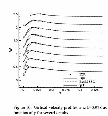
Reynolds stress equation model (RSM), also referred to as second moment closures are the most complete classical turbulence model. In these models, the eddy-viscosity hypothesis is avoided and the individual components of the Reynolds stress tensor are directly computed. These models use the exact Reynolds stress transport equation for their formulation. They account for the directional effects of the Reynolds stresses and the complex interactions in turbulent flows. Reynolds stress models offer significantly better accuracy than eddy-viscosity based turbulence models, while being computationally cheaper than Direct Numerical Simulations (DNS) and Large Eddy Simulations.

References

Gatski, T.B. and Speziale, C.G., "On explicit algebraic stress models for complex turbulent flows". J. Fluid Mech.
Rung, T., "Entwicklung anisotroper Wirbelzähigkeitsbeziehungen mit Hilfe von Projektionstechniken", PHD-thesis, Technical University Berlin, 2000
Taulbee, D.B., "An improved algebraic Reynolds stress model and corresponding nonlinaer stress model", Phys. Fluids, 28, pp 2555–2561, 1992
Lübcke, H., Rung, T. and Thiele, F. "Prediction of the Spreading Mechanism of 3D Turbulent Wall Jets with Explicit Reynolds-Stress Closures", Eng. Turbulence Modelling and Experiments 5, Mallorca, 2002
Wallin, S. and Johansson, A.V., "A new explicit algebraic Reynolds stress turbulence model including an improved near-wall treatment", Flow Modelling and Turbulence Measurements IV
Taulbee, D.B., "An improved algebraic Reynolds stress model and corresponding nonlinear stress model"
Jongen, T. and Gatski, T.B., "General explicit algebraic stress relations and best approximations for three-dimensional flows", Int. J. Engineering Science

This page is based on this Wikipedia article
Text is available under the CC BY-SA 4.0 license; additional terms may apply.
Images, videos and audio are available under their respective licenses.