
Autocorrelation, sometimes known as serial correlation in the discrete time case, is the correlation of a signal with a delayed copy of itself as a function of delay. Informally, it is the similarity between observations of a random variable as a function of the time lag between them. The analysis of autocorrelation is a mathematical tool for finding repeating patterns, such as the presence of a periodic signal obscured by noise, or identifying the missing fundamental frequency in a signal implied by its harmonic frequencies. It is often used in signal processing for analyzing functions or series of values, such as time domain signals.
The weighted arithmetic mean is similar to an ordinary arithmetic mean, except that instead of each of the data points contributing equally to the final average, some data points contribute more than others. The notion of weighted mean plays a role in descriptive statistics and also occurs in a more general form in several other areas of mathematics.
In statistics, the Gauss–Markov theorem states that the ordinary least squares (OLS) estimator has the lowest sampling variance within the class of linear unbiased estimators, if the errors in the linear regression model are uncorrelated, have equal variances and expectation value of zero. The errors do not need to be normal, nor do they need to be independent and identically distributed. The requirement that the estimator be unbiased cannot be dropped, since biased estimators exist with lower variance. See, for example, the James–Stein estimator, ridge regression, or simply any degenerate estimator.

In statistics, originally in geostatistics, kriging or Kriging, also known as Gaussian process regression, is a method of interpolation based on Gaussian process governed by prior covariances. Under suitable assumptions of the prior, kriging gives the best linear unbiased prediction (BLUP) at unsampled locations. Interpolating methods based on other criteria such as smoothness may not yield the BLUP. The method is widely used in the domain of spatial analysis and computer experiments. The technique is also known as Wiener–Kolmogorov prediction, after Norbert Wiener and Andrey Kolmogorov.
In statistics, G-tests are likelihood-ratio or maximum likelihood statistical significance tests that are increasingly being used in situations where chi-squared tests were previously recommended.
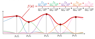
Inverse distance weighting (IDW) is a type of deterministic method for multivariate interpolation with a known scattered set of points. The assigned values to unknown points are calculated with a weighted average of the values available at the known points. This method can also be used to create spatial weights matrices in spatial autocorrelation analyses.

In the analysis of data, a correlogram is a chart of correlation statistics. For example, in time series analysis, a plot of the sample autocorrelations versus is an autocorrelogram. If cross-correlation is plotted, the result is called a cross-correlogram.
In statistics, a random effects model, also called a variance components model, is a statistical model where the model parameters are random variables. It is a kind of hierarchical linear model, which assumes that the data being analysed are drawn from a hierarchy of different populations whose differences relate to that hierarchy. A random effects model is a special case of a mixed model.
In statistics, the inverse Wishart distribution, also called the inverted Wishart distribution, is a probability distribution defined on real-valued positive-definite matrices. In Bayesian statistics it is used as the conjugate prior for the covariance matrix of a multivariate normal distribution.
An index of qualitative variation (IQV) is a measure of statistical dispersion in nominal distributions. Examples include the variation ratio or the information entropy.
GeoDa is a free software package that conducts spatial data analysis, geovisualization, spatial autocorrelation and spatial modeling.
Indicators of spatial association are statistics that evaluate the existence of clusters in the spatial arrangement of a given variable. For instance, if we are studying cancer rates among census tracts in a given city local clusters in the rates mean that there are areas that have higher or lower rates than is to be expected by chance alone; that is, the values occurring are above or below those of a random distribution in space.

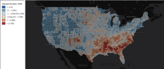
In statistics, Moran's I is a measure of spatial autocorrelation developed by Patrick Alfred Pierce Moran. Spatial autocorrelation is characterized by a correlation in a signal among nearby locations in space. Spatial autocorrelation is more complex than one-dimensional autocorrelation because spatial correlation is multi-dimensional and multi-directional.
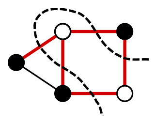
In a graph, a maximum cut is a cut whose size is at least the size of any other cut. That is, it is a partition of the graph's vertices into two complementary sets S and T, such that the number of edges between S and T is as large as possible. Finding such a cut is known as the max-cut problem.
The Technique for Order of Preference by Similarity to Ideal Solution (TOPSIS) is a multi-criteria decision analysis method, which was originally developed by Ching-Lai Hwang and Yoon in 1981 with further developments by Yoon in 1987, and Hwang, Lai and Liu in 1993. TOPSIS is based on the concept that the chosen alternative should have the shortest geometric distance from the positive ideal solution (PIS) and the longest geometric distance from the negative ideal solution (NIS). A dedicated book in the fuzzy context was published in 2021
Getis–Ord statistics, also known as Gi*, are used in spatial analysis to measure the local and global spatial autocorrelation. Developed by statisticians Arthur Getis and J. Keith Ord they are commonly used for Hot Spot Analysis to identify where features with high or low values are spatially clustered in a statistically significant way. Getis-Ord statistics are available in a number of software libraries such as CrimeStat, GeoDa, ArcGIS, PySAL and R.
Wartenberg's coefficient is a measure of correlation developed by epidemiologist Daniel Wartenberg. This coefficient is a multivariate extension of spatial autocorrelation that aims to account for spatial dependence of data while studying their covariance. A modified version of this statistic is available in the R package adespatial.
Lee's L is a bivariate spatial correlation coefficient which measures the association between two sets of observations made at the same spatial sites. Standard measures of association such as the Pearson correlation coefficient do not account for the spatial dimension of data, in particular they are vulnerable to inflation due to spatial autocorrelation. Lee's L is available in numerous spatial analysis software libraries including spdep and PySAL and has been applied in diverse applications such as studying air pollution, viticulture and housing rent.
Join count statistics are a method of spatial analysis used to assess the degree of association, in particular the autocorrelation, of categorical variables distributed over a spatial map. They were originally introduced by Australian statistician P. A. P. Moran. Join count statistics have found widespread use in econometrics, remote sensing and ecology. Join count statistics can be computed in a number of software packages including PASSaGE, GeoDA, PySAL and spdep.
The concept of a spatial weight is used in spatial analysis to describe neighbor relations between regions on a map. If location is a neighbor of location then otherwise . Usually we do not consider a site to be a neighbor of itself so . These coefficients are encoded in the spatial weight matrix


