A random variable is a mathematical formalization of a quantity or object which depends on random events. The term 'random variable' can be misleading as its mathematical definition is not actually random nor a variable, but rather it is a function from possible outcomes in a sample space to a measurable space, often to the real numbers.

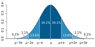
In probability theory, a probability density function (PDF), density function, or density of an absolutely continuous random variable, is a function whose value at any given sample in the sample space can be interpreted as providing a relative likelihood that the value of the random variable would be equal to that sample. Probability density is the probability per unit length, in other words, while the absolute likelihood for a continuous random variable to take on any particular value is 0, the value of the PDF at two different samples can be used to infer, in any particular draw of the random variable, how much more likely it is that the random variable would be close to one sample compared to the other sample.

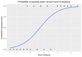
In statistics, the logistic model is a statistical model that models the log-odds of an event as a linear combination of one or more independent variables. In regression analysis, logistic regression is estimating the parameters of a logistic model. Formally, in binary logistic regression there is a single binary dependent variable, coded by an indicator variable, where the two values are labeled "0" and "1", while the independent variables can each be a binary variable or a continuous variable. The corresponding probability of the value labeled "1" can vary between 0 and 1, hence the labeling; the function that converts log-odds to probability is the logistic function, hence the name. The unit of measurement for the log-odds scale is called a logit, from logistic unit, hence the alternative names. See § Background and § Definition for formal mathematics, and § Example for a worked example.

In probability theory and statistics, the Gumbel distribution is used to model the distribution of the maximum of a number of samples of various distributions.
In statistics, Gibbs sampling or a Gibbs sampler is a Markov chain Monte Carlo (MCMC) algorithm for sampling from a specified multivariate probability distribution when direct sampling from the joint distribution is difficult, but sampling from the conditional distribution is more practical. This sequence can be used to approximate the joint distribution ; to approximate the marginal distribution of one of the variables, or some subset of the variables ; or to compute an integral. Typically, some of the variables correspond to observations whose values are known, and hence do not need to be sampled.
In mathematical analysis, asymptotic analysis, also known as asymptotics, is a method of describing limiting behavior.
In probability and statistics, a mixture distribution is the probability distribution of a random variable that is derived from a collection of other random variables as follows: first, a random variable is selected by chance from the collection according to given probabilities of selection, and then the value of the selected random variable is realized. The underlying random variables may be random real numbers, or they may be random vectors, in which case the mixture distribution is a multivariate distribution.
In statistics, a generalized linear model (GLM) is a flexible generalization of ordinary linear regression. The GLM generalizes linear regression by allowing the linear model to be related to the response variable via a link function and by allowing the magnitude of the variance of each measurement to be a function of its predicted value.

In probability theory, a distribution is said to be stable if a linear combination of two independent random variables with this distribution has the same distribution, up to location and scale parameters. A random variable is said to be stable if its distribution is stable. The stable distribution family is also sometimes referred to as the Lévy alpha-stable distribution, after Paul Lévy, the first mathematician to have studied it.
A continuous-time Markov chain (CTMC) is a continuous stochastic process in which, for each state, the process will change state according to an exponential random variable and then move to a different state as specified by the probabilities of a stochastic matrix. An equivalent formulation describes the process as changing state according to the least value of a set of exponential random variables, one for each possible state it can move to, with the parameters determined by the current state.

In probability theory and statistics, the probit function is the quantile function associated with the standard normal distribution. It has applications in data analysis and machine learning, in particular exploratory statistical graphics and specialized regression modeling of binary response variables.
In statistics, a tobit model is any of a class of regression models in which the observed range of the dependent variable is censored in some way. The term was coined by Arthur Goldberger in reference to James Tobin, who developed the model in 1958 to mitigate the problem of zero-inflated data for observations of household expenditure on durable goods. Because Tobin's method can be easily extended to handle truncated and other non-randomly selected samples, some authors adopt a broader definition of the tobit model that includes these cases.
In economics, discrete choice models, or qualitative choice models, describe, explain, and predict choices between two or more discrete alternatives, such as entering or not entering the labor market, or choosing between modes of transport. Such choices contrast with standard consumption models in which the quantity of each good consumed is assumed to be a continuous variable. In the continuous case, calculus methods can be used to determine the optimum amount chosen, and demand can be modeled empirically using regression analysis. On the other hand, discrete choice analysis examines situations in which the potential outcomes are discrete, such that the optimum is not characterized by standard first-order conditions. Thus, instead of examining "how much" as in problems with continuous choice variables, discrete choice analysis examines "which one". However, discrete choice analysis can also be used to examine the chosen quantity when only a few distinct quantities must be chosen from, such as the number of vehicles a household chooses to own and the number of minutes of telecommunications service a customer decides to purchase. Techniques such as logistic regression and probit regression can be used for empirical analysis of discrete choice.
In statistics, binomial regression is a regression analysis technique in which the response has a binomial distribution: it is the number of successes in a series of independent Bernoulli trials, where each trial has probability of success . In binomial regression, the probability of a success is related to explanatory variables: the corresponding concept in ordinary regression is to relate the mean value of the unobserved response to explanatory variables.

In probability theory, Dirichlet processes are a family of stochastic processes whose realizations are probability distributions. In other words, a Dirichlet process is a probability distribution whose range is itself a set of probability distributions. It is often used in Bayesian inference to describe the prior knowledge about the distribution of random variables—how likely it is that the random variables are distributed according to one or another particular distribution.

In probability and statistics, the quantile function outputs the value of a random variable such that its probability is less than or equal to an input probability value. Intuitively, the quantile function associates with a range at and below a probability input the likelihood that a random variable is realized in that range for some probability distribution. It is also called the percentile function, percent-point function or inverse cumulative distribution function.
In probability theory, the Mills ratio of a continuous random variable is the function
A geometric stable distribution or geo-stable distribution is a type of leptokurtic probability distribution. Geometric stable distributions were introduced in Klebanov, L. B., Maniya, G. M., and Melamed, I. A. (1985). A problem of Zolotarev and analogs of infinitely divisible and stable distributions in a scheme for summing a random number of random variables. These distributions are analogues for stable distributions for the case when the number of summands is random, independent of the distribution of summand, and having geometric distribution. The geometric stable distribution may be symmetric or asymmetric. A symmetric geometric stable distribution is also referred to as a Linnik distribution. The Laplace distribution and asymmetric Laplace distribution are special cases of the geometric stable distribution. The Mittag-Leffler distribution is also a special case of a geometric stable distribution.
In statistics, a zero-inflated model is a statistical model based on a zero-inflated probability distribution, i.e. a distribution that allows for frequent zero-valued observations.
In econometrics, the truncated normal hurdle model is a variant of the Tobit model and was first proposed by Cragg in 1971.


