In the theory of optimal binary search trees, the interleave lower bound is a lower bound on the number of operations required by a Binary Search Tree (BST) to execute a given sequence of accesses.
Several variants of this lower bound have been proven.[1][2][3] This article is based on a variation of the first Wilber's bound.[4] This lower bound is used in the design and analysis of Tango tree.[4] Furthermore, this lower bound can be rephrased and proven geometrically, Geometry of binary search trees.[5]
Definition
The bound is based on a fixed perfect BST, called the lower bound tree, over the keys . For example, for , can be represented by the following parenthesis structure:
[([1] 2 [3]) 4 ([5] 6 [7])]
For each node in , define:
to be the set of nodes in the left sub-tree of , including .
to be the set of nodes in the right sub-tree of .
Consider the following access sequence: . For a fixed node , and for each access , define the label of with respect to as:
"L" - if is in .
"R" - if is in ;
Null - otherwise.
The label of is the concatenation of the labels from all the accesses. For example, if the sequence of accesses is: then the label of the root is: "RRL", the label of 6 is: "RL", and the label of 2 is: "R".
For every node , define the amount of interleaving through y as the number of alternations between L and R in the label of . In the above example, the interleaving through and is and the interleaving through all other nodes is .
The interleave bound, , is the sum of the interleaving through all the nodes of the tree. The interleave bound of the above sequence is .
The Lower Bound Statement and its Proof
The interleave bound is summarized by the following theorem.
Theorem— Let be an access sequence. Denote by the interleave bound of , then is a lower bound of , the cost of optimal offline BST that serves .
Let be an access sequence. Denote by the state of an arbitrary BST at time i.e. after executing the sequence . We also fix a lower bound BST .
For a node in , define the transition point for at time to be the minimum-depth node in the BST such that the path from the root of to includes both a node from Left(y) and a node from Right(y). Intuitively, any BST algorithm on that accesses an element from Right(y) and then an element from Left(y) (or vice versa) must touch the transition point of at least once. In the following Lemma, we will show that transition point is well-defined.
Lemma 1—The transition point of a node in at a time exists and it is unique.[4]
Proof
Define to be the lowest common ancestor of all nodes in that are in Left(y). Given any two nodes in , the lowest common ancestor of and , denoted by , satisfies the following inequalities. . Consequently, is in Left(y), and is the unique node of minimum depth in . Same reasoning can be applied for , the lowest common ancestor of all nodes in that are in Right(y). In addition, the lowest common ancestor for all the points in Left(y) and right(y) is also in one of these sets. Therefore, the unique minimum depth node must be among the nodes of Left(y) and right(y). More precisely, it is either or . Suppose, it is . Then, is an ancestor of . Consequently, is a transition points since the path from the root to contains . Moreover, any path in from the root to a node in the sub-tree of must visit because it is the ancestor of all such nodes, and for any path to a node in the right region must visit because it is lowest common ancestor of all the nodes in right(y). To conclude, is the unique transition point for in .
The second lemma that we need to prove states that the transition point is stable. It will not change until it is touched.
Lemma 2—Given a node . Suppose is the transition point of at a time . If an access algorithm for a BST does not touch in for , then the transition point of will remain in for . [4]
Proof
Consider the same definition for and as in Lemma 1. Without loss of generality, suppose also that is an ancestor of in the BST at time , denoted by . As a result, will be the transition point of . By hypothesis, the BST algorithm does not touch the transition point, in our case , for the entirety of . Therefore, it does not touch any node in Right(y). Consequently, remains the lowest common ancestor for any two nodes in Right(y). However, the access algorithm might touch a node in Left(y). More precisely, it might touch the lowest common ancestor of all nodes in Left(y) at a time , which we will denoted by . Even so, will remain the ancestor of for the following reasons: Firstly, observe that any node of Left(y) that was outside the tree rooted at at time cannot enter this tree at a time , since isn't touched in this time frame. Secondly, there exists at least one node in Left(y) outside the tree rooted at , for any time . This is since was initially outside 's sub-tree, and no nodes from outside the tree can enter it in this timeframe. Now, consider . cannot be since is not in the sub-tree of . So, must be in Left(y), since . Consequently must be an ancestor of and by consequence an ancestor of at time . Therefore, there always exists a node in Left(y) on the path from the root to , and as such remains the transition point.
The last Lemma toward the proof states that every node has its unique transition point.
Lemma 3—Given a BST at time , , any node in can be only a transition for at most one node in .[4]
Proof
Given two distinct nodes . Let be the lowest common ancestor of respectively. From Lemma 1, we know that the transition point of is either or for . Now we have two main cases to consider.
Case 1: There is no ancestrally relation between and in . Consequently, the and are all disjoint. Thus, , and the transition points are different.
Case 2: Suppose without loss of generality that is an ancestor of in .
Case 2.1: Suppose that the transition point of is not in the tree rooted at in . Thus, it is different from and , and consequently the transition point of .
Case 2.2: The transition point of is in the tree rooted at in . More precisely, it is one of the lowest common ancestor of and . In other words, it is either or .
Suppose is the lowest common ancestor of the sub-tree rooted at and does not contain . We have and deeper than because one of them is the transition point. Suppose that is the transition point. Then, is less deep that . In this case, is the transition point of and is the transition point of . Similar reasoning applies if is less deep that . In sum, the transition point of is the less deep from and , and has the deeper one as a transition point.
In conclusion, the transition points are different in all the cases.
Now, we are ready to prove the theorem. First of all, observe that the number of touched transition points by the offline BST algorithm is a lower bound on its cost, we are counting less nodes than the required for the total cost.
We know by Lemma 3 that at any time , any node in can be only a transition for at most one node in . Thus, It is enough to count the number of touches of a transition node of , the sum over all .
Therefore, for a fixed node , let and to be defined as in Lemma 1. The transition point of is among these two nodes. In fact, it is the deeper one. Let be a maximal ordered access sequence to nodes that alternate between and . Then is the amount of interleaving through the node . Suppose that the even indexed accesses are in the , and the odd ones are in i.e. and . We know by the properties of lowest common ancestor that an access to a node in , it must touch . Similarly, an access to a node in must touch . Consider every . For two consecutive accesses and , if they avoid touching the access point of , then and must change in between. However, by Lemma 2, such change requires touching the transition point. Consequently, the BST access algorithm touches the transition point of at least once in the interval of . Summing over all , the best algorithm touches the transition point of at least . Summing over all ,
where is the amount of interleave through . By definition, the 's add up to . That concludes the proof.
In computer science, a binary search tree (BST), also called an ordered or sorted binary tree, is a rooted binary tree data structure with the key of each internal node being greater than all the keys in the respective node's left subtree and less than the ones in its right subtree. The time complexity of operations on the binary search tree is linear with respect to the height of the tree.
A hydrogen atom is an atom of the chemical element hydrogen. The electrically neutral hydrogen atom contains a nucleus of a single positively charged proton and a single negatively charged electron bound to the nucleus by the Coulomb force. Atomic hydrogen constitutes about 75% of the baryonic mass of the universe.
A splay tree is a binary search tree with the additional property that recently accessed elements are quick to access again. Like self-balancing binary search trees, a splay tree performs basic operations such as insertion, look-up and removal in O(log n) amortized time. For random access patterns drawn from a non-uniform random distribution, their amortized time can be faster than logarithmic, proportional to the entropy of the access pattern. For many patterns of non-random operations, also, splay trees can take better than logarithmic time, without requiring advance knowledge of the pattern. According to the unproven dynamic optimality conjecture, their performance on all access patterns is within a constant factor of the best possible performance that could be achieved by any other self-adjusting binary search tree, even one selected to fit that pattern. The splay tree was invented by Daniel Sleator and Robert Tarjan in 1985.
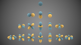
In mathematics and physical science, spherical harmonics are special functions defined on the surface of a sphere. They are often employed in solving partial differential equations in many scientific fields. The table of spherical harmonics contains a list of common spherical harmonics.
In the area of mathematics known as functional analysis, a reflexive space is a locally convex topological vector space for which the canonical evaluation map from into its bidual is a homeomorphism. A normed space is reflexive if and only if this canonical evaluation map is surjective, in which case this evaluation map is an isometric isomorphism and the normed space is a Banach space. Those spaces for which the canonical evaluation map is surjective are called semi-reflexive spaces.
In computer science, a disjoint-set data structure, also called a union–find data structure or merge–find set, is a data structure that stores a collection of disjoint (non-overlapping) sets. Equivalently, it stores a partition of a set into disjoint subsets. It provides operations for adding new sets, merging sets, and finding a representative member of a set. The last operation makes it possible to find out efficiently if any two elements are in the same or different sets.
In rotordynamics, the rigid rotor is a mechanical model of rotating systems. An arbitrary rigid rotor is a 3-dimensional rigid object, such as a top. To orient such an object in space requires three angles, known as Euler angles. A special rigid rotor is the linear rotor requiring only two angles to describe, for example of a diatomic molecule. More general molecules are 3-dimensional, such as water, ammonia, or methane.
In coding theory, the Kraft–McMillan inequality gives a necessary and sufficient condition for the existence of a prefix code or a uniquely decodable code for a given set of codeword lengths. Its applications to prefix codes and trees often find use in computer science and information theory. The prefix code can contain either finitely many or infinitely many codewords.
In quantum physics, the spin–orbit interaction is a relativistic interaction of a particle's spin with its motion inside a potential. A key example of this phenomenon is the spin–orbit interaction leading to shifts in an electron's atomic energy levels, due to electromagnetic interaction between the electron's magnetic dipole, its orbital motion, and the electrostatic field of the positively charged nucleus. This phenomenon is detectable as a splitting of spectral lines, which can be thought of as a Zeeman effect product of two relativistic effects: the apparent magnetic field seen from the electron perspective and the magnetic moment of the electron associated with its intrinsic spin. A similar effect, due to the relationship between angular momentum and the strong nuclear force, occurs for protons and neutrons moving inside the nucleus, leading to a shift in their energy levels in the nucleus shell model. In the field of spintronics, spin–orbit effects for electrons in semiconductors and other materials are explored for technological applications. The spin–orbit interaction is at the origin of magnetocrystalline anisotropy and the spin Hall effect.
In queueing theory, a discipline within the mathematical theory of probability, a Jackson network is a class of queueing network where the equilibrium distribution is particularly simple to compute as the network has a product-form solution. It was the first significant development in the theory of networks of queues, and generalising and applying the ideas of the theorem to search for similar product-form solutions in other networks has been the subject of much research, including ideas used in the development of the Internet. The networks were first identified by James R. Jackson and his paper was re-printed in the journal Management Science’s ‘Ten Most Influential Titles of Management Sciences First Fifty Years.’
The Wigner D-matrix is a unitary matrix in an irreducible representation of the groups SU(2) and SO(3). It was introduced in 1927 by Eugene Wigner, and plays a fundamental role in the quantum mechanical theory of angular momentum. The complex conjugate of the D-matrix is an eigenfunction of the Hamiltonian of spherical and symmetric rigid rotors. The letter D stands for Darstellung, which means "representation" in German.
In metric geometry, the metric envelope or tight span of a metric space M is an injective metric space into which M can be embedded. In some sense it consists of all points "between" the points of M, analogous to the convex hull of a point set in a Euclidean space. The tight span is also sometimes known as the injective envelope or hyperconvex hull of M. It has also been called the injective hull, but should not be confused with the injective hull of a module in algebra, a concept with a similar description relative to the category of R-modules rather than metric spaces.
In functional analysis, the dual norm is a measure of size for a continuous linear function defined on a normed vector space.
In mathematics, particularly numerical analysis, the Bramble–Hilbert lemma, named after James H. Bramble and Stephen Hilbert, bounds the error of an approximation of a function by a polynomial of order at most in terms of derivatives of of order . Both the error of the approximation and the derivatives of are measured by norms on a bounded domain in . This is similar to classical numerical analysis, where, for example, the error of linear interpolation can be bounded using the second derivative of . However, the Bramble–Hilbert lemma applies in any number of dimensions, not just one dimension, and the approximation error and the derivatives of are measured by more general norms involving averages, not just the maximum norm.
In mathematics, discrete Chebyshev polynomials, or Gram polynomials, are a type of discrete orthogonal polynomials used in approximation theory, introduced by Pafnuty Chebyshev and rediscovered by Gram. They were later found to be applicable to various algebraic properties of spin angular momentum.
The Priority R-tree is a worst-case asymptotically optimal alternative to the spatial tree R-tree. It was first proposed by Arge, De Berg, Haverkort and Yi, K. in an article from 2004. The prioritized R-tree is essentially a hybrid between a k-dimensional tree and a R-tree in that it defines a given object's N-dimensional bounding volume as a point in N-dimensions, represented by the ordered pair of the rectangles. The term prioritized arrives from the introduction of four priority-leaves that represents the most extreme values of each dimensions, included in every branch of the tree. Before answering a window-query by traversing the sub-branches, the prioritized R-tree first checks for overlap in its priority nodes. The sub-branches are traversed by checking whether the least value of the first dimension of the query is above the value of the sub-branches. This gives access to a quick indexation by the value of the first dimension of the bounding box.
In computer science, the range query problem consists of efficiently answering several queries regarding a given interval of elements within an array. For example, a common task, known as range minimum query, is finding the smallest value inside a given range within a list of numbers.
In computer science, one approach to the dynamic optimality problem on online algorithms for binary search trees involves reformulating the problem geometrically, in terms of augmenting a set of points in the plane with as few additional points as possible to avoid rectangles with only two points on their boundary.
In coding theory, burst error-correcting codes employ methods of correcting burst errors, which are errors that occur in many consecutive bits rather than occurring in bits independently of each other.
In computer science, an optimal binary search tree (Optimal BST), sometimes called a weight-balanced binary tree, is a binary search tree which provides the smallest possible search time (or expected search time) for a given sequence of accesses (or access probabilities). Optimal BSTs are generally divided into two types: static and dynamic.
References
↑ Wilber, R. (1989). "Lower Bounds for Accessing Binary Search Trees with Rotations". SIAM Journal on Computing. 18: 56–67. doi:10.1137/0218004.
↑ Hampapuram, H.; Fredman, M. L. (1998). "Optimal Biweighted Binary Trees and the Complexity of Maintaining Partial Sums". SIAM Journal on Computing. 28: 1–9. doi:10.1137/S0097539795291598.
This page is based on this Wikipedia article Text is available under the CC BY-SA 4.0 license; additional terms may apply. Images, videos and audio are available under their respective licenses.