Related Research Articles
A hidden Markov model (HMM) is a Markov model in which the observations are dependent on a latent Markov process. An HMM requires that there be an observable process whose outcomes depend on the outcomes of in a known way. Since cannot be observed directly, the goal is to learn about state of by observing . By definition of being a Markov model, an HMM has an additional requirement that the outcome of at time must be "influenced" exclusively by the outcome of at and that the outcomes of and at must be conditionally independent of at given at time . Estimation of the parameters in an HMM can be performed using maximum likelihood estimation. For linear chain HMMs, the Baum–Welch algorithm can be used to estimate parameters.
A Bayesian network is a probabilistic graphical model that represents a set of variables and their conditional dependencies via a directed acyclic graph (DAG). While it is one of several forms of causal notation, causal networks are special cases of Bayesian networks. Bayesian networks are ideal for taking an event that occurred and predicting the likelihood that any one of several possible known causes was the contributing factor. For example, a Bayesian network could represent the probabilistic relationships between diseases and symptoms. Given symptoms, the network can be used to compute the probabilities of the presence of various diseases.
The Viterbi algorithm is a dynamic programming algorithm for obtaining the maximum a posteriori probability estimate of the most likely sequence of hidden states—called the Viterbi path—that results in a sequence of observed events. This is done especially in the context of Markov information sources and hidden Markov models (HMM).
A graphical model or probabilistic graphical model (PGM) or structured probabilistic model is a probabilistic model for which a graph expresses the conditional dependence structure between random variables. They are commonly used in probability theory, statistics—particularly Bayesian statistics—and machine learning.
In statistics, Gibbs sampling or a Gibbs sampler is a Markov chain Monte Carlo (MCMC) algorithm for sampling from a specified multivariate probability distribution when direct sampling from the joint distribution is difficult, but sampling from the conditional distribution is more practical. This sequence can be used to approximate the joint distribution ; to approximate the marginal distribution of one of the variables, or some subset of the variables ; or to compute an integral. Typically, some of the variables correspond to observations whose values are known, and hence do not need to be sampled.
In computer science, a selection algorithm is an algorithm for finding the th smallest value in a collection of ordered values, such as numbers. The value that it finds is called the th order statistic. Selection includes as special cases the problems of finding the minimum, median, and maximum element in the collection. Selection algorithms include quickselect, and the median of medians algorithm. When applied to a collection of values, these algorithms take linear time, as expressed using big O notation. For data that is already structured, faster algorithms may be possible; as an extreme case, selection in an already-sorted array takes time .
Belief propagation, also known as sum–product message passing, is a message-passing algorithm for performing inference on graphical models, such as Bayesian networks and Markov random fields. It calculates the marginal distribution for each unobserved node, conditional on any observed nodes. Belief propagation is commonly used in artificial intelligence and information theory, and has demonstrated empirical success in numerous applications, including low-density parity-check codes, turbo codes, free energy approximation, and satisfiability.
The forward algorithm, in the context of a hidden Markov model (HMM), is used to calculate a 'belief state': the probability of a state at a certain time, given the history of evidence. The process is also known as filtering. The forward algorithm is closely related to, but distinct from, the Viterbi algorithm.
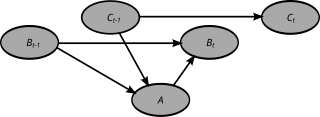
A dynamic Bayesian network (DBN) is a Bayesian network (BN) which relates variables to each other over adjacent time steps.
In the domain of physics and probability, a Markov random field (MRF), Markov network or undirected graphical model is a set of random variables having a Markov property described by an undirected graph. In other words, a random field is said to be a Markov random field if it satisfies Markov properties. The concept originates from the Sherrington–Kirkpatrick model.
A factor graph is a bipartite graph representing the factorization of a function. In probability theory and its applications, factor graphs are used to represent factorization of a probability distribution function, enabling efficient computations, such as the computation of marginal distributions through the sum–product algorithm. One of the important success stories of factor graphs and the sum–product algorithm is the decoding of capacity-approaching error-correcting codes, such as LDPC and turbo codes.
A Markov logic network (MLN) is a probabilistic logic which applies the ideas of a Markov network to first-order logic, defining probability distributions on possible worlds on any given domain.

In computer science, recursion is a method of solving a computational problem where the solution depends on solutions to smaller instances of the same problem. Recursion solves such recursive problems by using functions that call themselves from within their own code. The approach can be applied to many types of problems, and recursion is one of the central ideas of computer science.
The power of recursion evidently lies in the possibility of defining an infinite set of objects by a finite statement. In the same manner, an infinite number of computations can be described by a finite recursive program, even if this program contains no explicit repetitions.

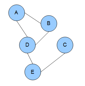
In graph theory, a moral graph is used to find the equivalent undirected form of a directed acyclic graph. It is a key step of the junction tree algorithm, used in belief propagation on graphical models.

The junction tree algorithm is a method used in machine learning to extract marginalization in general graphs. In essence, it entails performing belief propagation on a modified graph called a junction tree. The graph is called a tree because it branches into different sections of data; nodes of variables are the branches. The basic premise is to eliminate cycles by clustering them into single nodes. Multiple extensive classes of queries can be compiled at the same time into larger structures of data. There are different algorithms to meet specific needs and for what needs to be calculated. Inference algorithms gather new developments in the data and calculate it based on the new information provided.
In distributed computing, leader election is the process of designating a single process as the organizer of some task distributed among several computers (nodes). Before the task has begun, all network nodes are either unaware which node will serve as the "leader" of the task, or unable to communicate with the current coordinator. After a leader election algorithm has been run, however, each node throughout the network recognizes a particular, unique node as the task leader.
Hierarchical temporal memory (HTM) is a biologically constrained machine intelligence technology developed by Numenta. Originally described in the 2004 book On Intelligence by Jeff Hawkins with Sandra Blakeslee, HTM is primarily used today for anomaly detection in streaming data. The technology is based on neuroscience and the physiology and interaction of pyramidal neurons in the neocortex of the mammalian brain.
Pointer jumping or path doubling is a design technique for parallel algorithms that operate on pointer structures, such as linked lists and directed graphs. Pointer jumping allows an algorithm to follow paths with a time complexity that is logarithmic with respect to the length of the longest path. It does this by "jumping" to the end of the path computed by neighbors.
The following outline is provided as an overview of and topical guide to machine learning:
In network theory, collective classification is the simultaneous prediction of the labels for multiple objects, where each label is predicted using information about the object's observed features, the observed features and labels of its neighbors, and the unobserved labels of its neighbors. Collective classification problems are defined in terms of networks of random variables, where the network structure determines the relationship between the random variables. Inference is performed on multiple random variables simultaneously, typically by propagating information between nodes in the network to perform approximate inference. Approaches that use collective classification can make use of relational information when performing inference. Examples of collective classification include predicting attributes of individuals in a social network, classifying webpages in the World Wide Web, and inferring the research area of a paper in a scientific publication dataset.
References
- ↑ J. Binder, K. Murphy and S. Russell. Space-Efficient Inference in Dynamic Probabilistic Networks. Int'l, Joint Conf. on Artificial Intelligence, 1997.