A histogram is a visual representation of the distribution of quantitative data. The term was first introduced by Karl Pearson. To construct a histogram, the first step is to "bin" the range of values— divide the entire range of values into a series of intervals—and then count how many values fall into each interval. The bins are usually specified as consecutive, non-overlapping intervals of a variable. The bins (intervals) are adjacent and are typically of equal size.

Idempotence is the property of certain operations in mathematics and computer science whereby they can be applied multiple times without changing the result beyond the initial application. The concept of idempotence arises in a number of places in abstract algebra and functional programming.

The median of a set of numbers is the value separating the higher half from the lower half of a data sample, a population, or a probability distribution. For a data set, it may be thought of as the “middle" value. The basic feature of the median in describing data compared to the mean is that it is not skewed by a small proportion of extremely large or small values, and therefore provides a better representation of the center. Median income, for example, may be a better way to describe the center of the income distribution because increases in the largest incomes alone have no effect on the median. For this reason, the median is of central importance in robust statistics.

Pulse-width modulation (PWM), also known as pulse-duration modulation (PDM) or pulse-length modulation (PLM), is any method of representing a signal as a rectangular wave with a varying duty cycle.
An inverse problem in science is the process of calculating from a set of observations the causal factors that produced them: for example, calculating an image in X-ray computed tomography, source reconstruction in acoustics, or calculating the density of the Earth from measurements of its gravity field. It is called an inverse problem because it starts with the effects and then calculates the causes. It is the inverse of a forward problem, which starts with the causes and then calculates the effects.
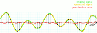
Quantization, in mathematics and digital signal processing, is the process of mapping input values from a large set to output values in a (countable) smaller set, often with a finite number of elements. Rounding and truncation are typical examples of quantization processes. Quantization is involved to some degree in nearly all digital signal processing, as the process of representing a signal in digital form ordinarily involves rounding. Quantization also forms the core of essentially all lossy compression algorithms.
Edge detection includes a variety of mathematical methods that aim at identifying edges, defined as curves in a digital image at which the image brightness changes sharply or, more formally, has discontinuities. The same problem of finding discontinuities in one-dimensional signals is known as step detection and the problem of finding signal discontinuities over time is known as change detection. Edge detection is a fundamental tool in image processing, machine vision and computer vision, particularly in the areas of feature detection and feature extraction.
In time series analysis, dynamic time warping (DTW) is an algorithm for measuring similarity between two temporal sequences, which may vary in speed. For instance, similarities in walking could be detected using DTW, even if one person was walking faster than the other, or if there were accelerations and decelerations during the course of an observation. DTW has been applied to temporal sequences of video, audio, and graphics data — indeed, any data that can be turned into a one-dimensional sequence can be analyzed with DTW. A well-known application has been automatic speech recognition, to cope with different speaking speeds. Other applications include speaker recognition and online signature recognition. It can also be used in partial shape matching applications.

In the study of dynamical systems, a delay embedding theorem gives the conditions under which a chaotic dynamical system can be reconstructed from a sequence of observations of the state of that system. The reconstruction preserves the properties of the dynamical system that do not change under smooth coordinate changes, but it does not preserve the geometric shape of structures in phase space.
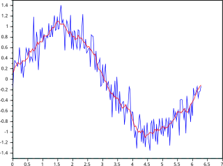
In statistics, a moving average is a calculation to analyze data points by creating a series of averages of different selections of the full data set. Variations include: simple, cumulative, or weighted forms.
In signal processing, a nonlinearfilter is a filter whose output is not a linear function of its input. That is, if the filter outputs signals R and S for two input signals r and s separately, but does not always output αR + βS when the input is a linear combination αr + βs.

Geometry processing is an area of research that uses concepts from applied mathematics, computer science and engineering to design efficient algorithms for the acquisition, reconstruction, analysis, manipulation, simulation and transmission of complex 3D models. As the name implies, many of the concepts, data structures, and algorithms are directly analogous to signal processing and image processing. For example, where image smoothing might convolve an intensity signal with a blur kernel formed using the Laplace operator, geometric smoothing might be achieved by convolving a surface geometry with a blur kernel formed using the Laplace-Beltrami operator.
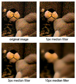
The median filter is a non-linear digital filtering technique, often used to remove noise from an image or signal. Such noise reduction is a typical pre-processing step to improve the results of later processing. Median filtering is very widely used in digital image processing because, under certain conditions, it preserves edges while removing noise, also having applications in signal processing.
In statistics, M-estimators are a broad class of extremum estimators for which the objective function is a sample average. Both non-linear least squares and maximum likelihood estimation are special cases of M-estimators. The definition of M-estimators was motivated by robust statistics, which contributed new types of M-estimators. However, M-estimators are not inherently robust, as is clear from the fact that they include maximum likelihood estimators, which are in general not robust. The statistical procedure of evaluating an M-estimator on a data set is called M-estimation.

In time series analysis, singular spectrum analysis (SSA) is a nonparametric spectral estimation method. It combines elements of classical time series analysis, multivariate statistics, multivariate geometry, dynamical systems and signal processing. Its roots lie in the classical Karhunen (1946)–Loève spectral decomposition of time series and random fields and in the Mañé (1981)–Takens (1981) embedding theorem. SSA can be an aid in the decomposition of time series into a sum of components, each having a meaningful interpretation. The name "singular spectrum analysis" relates to the spectrum of eigenvalues in a singular value decomposition of a covariance matrix, and not directly to a frequency domain decomposition.
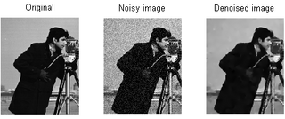
In signal processing, particularly image processing, total variation denoising, also known as total variation regularization or total variation filtering, is a noise removal process (filter). It is based on the principle that signals with excessive and possibly spurious detail have high total variation, that is, the integral of the image gradient magnitude is high. According to this principle, reducing the total variation of the signal—subject to it being a close match to the original signal—removes unwanted detail whilst preserving important details such as edges. The concept was pioneered by L. I. Rudin, S. Osher, and E. Fatemi in 1992 and so is today known as the ROF model.

In statistics and signal processing, step detection is the process of finding abrupt changes in the mean level of a time series or signal. It is usually considered as a special case of the statistical method known as change detection or change point detection. Often, the step is small and the time series is corrupted by some kind of noise, and this makes the problem challenging because the step may be hidden by the noise. Therefore, statistical and/or signal processing algorithms are often required.
The Landweber iteration or Landweber algorithm is an algorithm to solve ill-posed linear inverse problems, and it has been extended to solve non-linear problems that involve constraints. The method was first proposed in the 1950s by Louis Landweber, and it can be now viewed as a special case of many other more general methods.
System identification is a method of identifying or measuring the mathematical model of a system from measurements of the system inputs and outputs. The applications of system identification include any system where the inputs and outputs can be measured and include industrial processes, control systems, economic data, biology and the life sciences, medicine, social systems and many more.
In signal processing, multidimensional empirical mode decomposition is an extension of the one-dimensional (1-D) EMD algorithm to a signal encompassing multiple dimensions. The Hilbert–Huang empirical mode decomposition (EMD) process decomposes a signal into intrinsic mode functions combined with the Hilbert spectral analysis, known as the Hilbert–Huang transform (HHT). The multidimensional EMD extends the 1-D EMD algorithm into multiple-dimensional signals. This decomposition can be applied to image processing, audio signal processing, and various other multidimensional signals.


