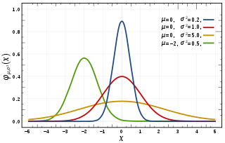
A normal distribution is a probability distribution used to model phenomena that have a default behaviour and cumulative possible deviations from that behaviour. For instance, a proficient archer's arrows are expected to land around the bull's eye of the target; however, due to aggregating imperfections in the archer's technique, most arrows will miss the bull's eye by some distance. The average of this distance is known in archery as accuracy, while the amount of variation in the distances as precision. In the context of a normal distribution, accuracy and precision are referred to as the mean and the standard deviation, respectively. Thus, a narrow measure of an archer's proficiency can be expressed with two values: a mean and a standard deviation. In a normal distribution, these two values mean: there is a ~68% probability that an arrow will land within one standard deviation of the archer's average accuracy; a ~95% probability that an arrow will land within two standard deviations of the archer's average accuracy; ~99.7% within three; and so on, slowly increasing towards 100%.
In probability theory, the central limit theorem (CLT) establishes that, in many situations, when independent random variables are summed up, their properly normalized sum tends toward a normal distribution even if the original variables themselves are not normally distributed.

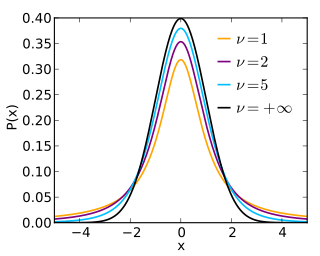
In probability and statistics, Student's t-distribution is any member of a family of continuous probability distributions that arise when estimating the mean of a normally distributed population in situations where the sample size is small and the population's standard deviation is unknown. It was developed by English statistician William Sealy Gosset under the pseudonym "Student".
In the mathematical field of real analysis, the monotone convergence theorem is any of a number of related theorems proving the convergence of monotonic sequences that are also bounded. Informally, the theorems state that if a sequence is increasing and bounded above by a supremum, then the sequence will converge to the supremum; in the same way, if a sequence is decreasing and is bounded below by an infimum, it will converge to the infimum.

In mathematics, the Wiener process is a real valued continuous-time stochastic process named in honor of American mathematician Norbert Wiener for his investigations on the mathematical properties of the one-dimensional Brownian motion. It is often also called Brownian motion due to its historical connection with the physical process of the same name originally observed by Scottish botanist Robert Brown. It is one of the best known Lévy processes and occurs frequently in pure and applied mathematics, economics, quantitative finance, evolutionary biology, and physics.

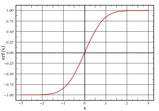
In mathematics, the error function, often denoted by erf, is a complex function of a complex variable defined as:

In probability theory, a martingale is a sequence of random variables for which, at a particular time, the conditional expectation of the next value in the sequence is equal to the present value, regardless of all prior values.
In probability theory and statistics, a Gaussian process is a stochastic process, such that every finite collection of those random variables has a multivariate normal distribution, i.e. every finite linear combination of them is normally distributed. The distribution of a Gaussian process is the joint distribution of all those random variables, and as such, it is a distribution over functions with a continuous domain, e.g. time or space.

In probability theory, in particular in the study of stochastic processes, a stopping time is a specific type of “random time”: a random variable whose value is interpreted as the time at which a given stochastic process exhibits a certain behavior of interest. A stopping time is often defined by a stopping rule, a mechanism for deciding whether to continue or stop a process on the basis of the present position and past events, and which will almost always lead to a decision to stop at some finite time.

The scaled inverse chi-squared distribution is the distribution for x = 1/s2, where s2 is a sample mean of the squares of ν independent normal random variables that have mean 0 and inverse variance 1/σ2 = τ2. The distribution is therefore parametrised by the two quantities ν and τ2, referred to as the number of chi-squared degrees of freedom and the scaling parameter, respectively.
In mathematics, the Stolz–Cesàro theorem is a criterion for proving the convergence of a sequence. The theorem is named after mathematicians Otto Stolz and Ernesto Cesàro, who stated and proved it for the first time.

Oblate spheroidal coordinates are a three-dimensional orthogonal coordinate system that results from rotating the two-dimensional elliptic coordinate system about the non-focal axis of the ellipse, i.e., the symmetry axis that separates the foci. Thus, the two foci are transformed into a ring of radius in the x-y plane. Oblate spheroidal coordinates can also be considered as a limiting case of ellipsoidal coordinates in which the two largest semi-axes are equal in length.
In mathematics, the theory of optimal stopping or early stopping is concerned with the problem of choosing a time to take a particular action, in order to maximise an expected reward or minimise an expected cost. Optimal stopping problems can be found in areas of statistics, economics, and mathematical finance. A key example of an optimal stopping problem is the secretary problem. Optimal stopping problems can often be written in the form of a Bellman equation, and are therefore often solved using dynamic programming.
In mathematics, a local martingale is a type of stochastic process, satisfying the localized version of the martingale property. Every martingale is a local martingale; every bounded local martingale is a martingale; in particular, every local martingale that is bounded from below is a supermartingale, and every local martingale that is bounded from above is a submartingale; however, in general a local martingale is not a martingale, because its expectation can be distorted by large values of small probability. In particular, a driftless diffusion process is a local martingale, but not necessarily a martingale.
Continuous wavelets of compact support can be built, which are related to the beta distribution. The process is derived from probability distributions using blur derivative. These new wavelets have just one cycle, so they are termed unicycle wavelets. They can be viewed as a soft variety of Haar wavelets whose shape is fine-tuned by two parameters and . Closed-form expressions for beta wavelets and scale functions as well as their spectra are derived. Their importance is due to the Central Limit Theorem by Gnedenko and Kolmogorov applied for compactly supported signals.
Expected shortfall (ES) is a risk measure—a concept used in the field of financial risk measurement to evaluate the market risk or credit risk of a portfolio. The "expected shortfall at q% level" is the expected return on the portfolio in the worst of cases. ES is an alternative to value at risk that is more sensitive to the shape of the tail of the loss distribution.

In probability theory and statistics, the Conway–Maxwell–Poisson distribution is a discrete probability distribution named after Richard W. Conway, William L. Maxwell, and Siméon Denis Poisson that generalizes the Poisson distribution by adding a parameter to model overdispersion and underdispersion. It is a member of the exponential family, has the Poisson distribution and geometric distribution as special cases and the Bernoulli distribution as a limiting case.

Anatoly Alexeyevich Karatsuba was a Russian mathematician working in the field of analytic number theory, p-adic numbers and Dirichlet series.
In probability a quasi-stationary distribution is a random process that admits one or several absorbing states that are reached almost surely, but is initially distributed such that it can evolve for a long time without reaching it. The most common example is the evolution of a population: the only equilibrium is when there is no one left, but if we model the number of people it is likely to remain stable for a long period of time before it eventually collapses.
In differential geometry, Santaló's formula describes how to integrate a function on the unit sphere bundle of a Riemannian manifold by first integrating along every geodesic separately and then over the space of all geodesics. It is a standard tool in integral geometry and has applications in isoperimetric and rigidity results. The formula is named after Luis Santaló, who first proved the result in 1952.
Note, however, that the proof of Theorem 5.4 in Hall & Heyde contains an error. For further discussion, see


