In probability theory, the central limit theorem (CLT) states that, under appropriate conditions, the distribution of a normalized version of the sample mean converges to a standard normal distribution. This holds even if the original variables themselves are not normally distributed. There are several versions of the CLT, each applying in the context of different conditions.
The theorem is a key concept in probability theory because it implies that probabilistic and statistical methods that work for normal distributions can be applicable to many problems involving other types of distributions.
This theorem has seen many changes during the formal development of probability theory. Previous versions of the theorem date back to 1811, but in its modern form it was only precisely stated in the 1920s.[1]
In other words, suppose that a large sample of observations is obtained, each observation being randomly produced in a way that does not depend on the values of the other observations, and the average (arithmetic mean) of the observed values is computed. If this procedure is performed many times, resulting in a collection of observed averages, the central limit theorem says that if the sample size is large enough, the probability distribution of these averages will closely approximate a normal distribution.
The central limit theorem has several variants. In its common form, the random variables must be independent and identically distributed (i.i.d.). This requirement can be weakened; convergence of the mean to the normal distribution also occurs for non-identical distributions or for non-independent observations if they comply with certain conditions.
Whatever the form of the population distribution, the sampling distribution tends to a Gaussian, and its dispersion is given by the central limit theorem.
The classical central limit theorem describes the size and the distributional form of the stochastic fluctuations around the deterministic number during this convergence. More precisely, it states that as gets larger, the distribution of the normalized mean , i.e. the difference between the sample average and its limit scaled by the factor , approaches the normal distribution with mean and variance For large enough the distribution of gets arbitrarily close to the normal distribution with mean and variance
The usefulness of the theorem is that the distribution of approaches normality regardless of the shape of the distribution of the individual Formally, the theorem can be stated as follows:
Lindeberg–Lévy CLT—Suppose is a sequence of i.i.d. random variables with and Then, as approaches infinity, the random variables converge in distribution to a normal:[4]
In the case convergence in distribution means that the cumulative distribution functions of converge pointwise to the cdf of the distribution: for every real number
where is the standard normal cdf evaluated at The convergence is uniform in in the sense that
where denotes the least upper bound (or supremum) of the set.[5]
Lyapunov CLT
In this variant of the central limit theorem the random variables have to be independent, but not necessarily identically distributed. The theorem also requires that random variables have moments of some order , and that the rate of growth of these moments is limited by the Lyapunov condition given below.
Lyapunov CLT[6]—Suppose is a sequence of independent random variables, each with finite expected value and variance . Define
If for some ,Lyapunov’s condition
is satisfied, then a sum of converges in distribution to a standard normal random variable, as goes to infinity:
In practice it is usually easiest to check Lyapunov's condition for .
If a sequence of random variables satisfies Lyapunov's condition, then it also satisfies Lindeberg's condition. The converse implication, however, does not hold.
In the same setting and with the same notation as above, the Lyapunov condition can be replaced with the following weaker one (from Lindeberg in 1920).
Suppose that for every ,
where is the indicator function. Then the distribution of the standardized sums
converges towards the standard normal distribution .
CLT for the sum of a random number of random variables
Rather than summing an integer number of random variables and taking , the sum can be of a random number of random variables, with conditions on . For example, the following theorem is Corollary 4 of Robbins (1948). It assumes that is asymptotically normal (Robbins also developed other conditions that lead to the same result).
Robbins CLT[7][8]—Let be independent, identically distributed random variables with and , and let be a sequence of non-negative integer-valued random variables that are independent of . Assume for each that and
where denotes convergence in distribution and is the normal distribution with mean 0, variance 1. Then
Multidimensional CLT
Proofs that use characteristic functions can be extended to cases where each individual is a random vector in , with mean vector and covariance matrix (among the components of the vector), and these random vectors are independent and identically distributed. The multidimensional central limit theorem states that when scaled, sums converge to a multivariate normal distribution.[9] Summation of these vectors is done component-wise.
For let
be independent random vectors. The sum of the random vectors is
and their average is
Therefore,
The multivariate central limit theorem states that
The rate of convergence is given by the following Berry–Esseen type result:
Theorem[10]—Let be independent -valued random vectors, each having mean zero. Write and assume is invertible. Let be a -dimensional Gaussian with the same mean and same covariance matrix as . Then for all convex sets ,
where is a universal constant, , and denotes the Euclidean norm on .
It is unknown whether the factor is necessary.[11]
The generalized central limit theorem
The generalized central limit theorem (GCLT) was an effort of multiple mathematicians (Bernstein, Lindeberg, Lévy, Feller, Kolmogorov, and others) over the period from 1920 to 1937.[12] The first published complete proof of the GCLT was in 1937 by Paul Lévy in French.[13] An English language version of the complete proof of the GCLT is available in the translation of Gnedenko and Kolmogorov's 1954 book.[14]
Statement of GCLT—A non-degenerate random variable Z is α-stable for some 0 < α ≤ 2 if and only if there is an independent, identically distributed sequence of random variables X1, X2, X3,..., and constants an > 0, bn ∈ ℝ with Here, '→' means the sequence of random variable sums converges in distribution; i.e., the corresponding distributions satisfy Fn(y) → F(y) at all continuity points of F.
In other words, if sums of independent, identically distributed random variables converge in distribution to some Z, then Z must be a stable distribution.
Dependent processes
CLT under weak dependence
A useful generalization of a sequence of independent, identically distributed random variables is a mixing random process in discrete time; "mixing" means, roughly, that random variables temporally far apart from one another are nearly independent. Several kinds of mixing are used in ergodic theory and probability theory. See especially strong mixing (also called α-mixing) defined by where is so-called strong mixing coefficient.
A simplified formulation of the central limit theorem under strong mixing is:[16]
Theorem—Suppose that is stationary and -mixing with and that and . Denote , then the limit
exists, and if then converges in distribution to .
In fact,
where the series converges absolutely.
The assumption cannot be omitted, since the asymptotic normality fails for where are another stationary sequence.
There is a stronger version of the theorem:[17] the assumption is replaced with , and the assumption is replaced with
Existence of such ensures the conclusion. For encyclopedic treatment of limit theorems under mixing conditions see (Bradley 2007).
Assume are independent and identically distributed random variables, each with mean and finite variance . The sum has mean and variance. Consider the random variable
where in the last step we defined the new random variables , each with zero mean and unit variance (). The characteristic function of is given by
where in the last step we used the fact that all of the are identically distributed. The characteristic function of is, by Taylor's theorem,
where is "little o notation" for some function of that goes to zero more rapidly than . By the limit of the exponential function(), the characteristic function of equals
All of the higher order terms vanish in the limit . The right hand side equals the characteristic function of a standard normal distribution , which implies through Lévy's continuity theorem that the distribution of will approach as . Therefore, the sample average
is such that
converges to the normal distribution , from which the central limit theorem follows.
Convergence to the limit
The central limit theorem gives only an asymptotic distribution. As an approximation for a finite number of observations, it provides a reasonable approximation only when close to the peak of the normal distribution; it requires a very large number of observations to stretch into the tails.[citation needed]
The convergence in the central limit theorem is uniform because the limiting cumulative distribution function is continuous. If the third central moment exists and is finite, then the speed of convergence is at least on the order of (see Berry–Esseen theorem). Stein's method[21] can be used not only to prove the central limit theorem, but also to provide bounds on the rates of convergence for selected metrics.[22]
The convergence to the normal distribution is monotonic, in the sense that the entropy of increases monotonically to that of the normal distribution.[23]
The central limit theorem applies in particular to sums of independent and identically distributed discrete random variables. A sum of discrete random variables is still a discrete random variable, so that we are confronted with a sequence of discrete random variables whose cumulative probability distribution function converges towards a cumulative probability distribution function corresponding to a continuous variable (namely that of the normal distribution). This means that if we build a histogram of the realizations of the sum of n independent identical discrete variables, the piecewise-linear curve that joins the centers of the upper faces of the rectangles forming the histogram converges toward a Gaussian curve as n approaches infinity; this relation is known as de Moivre–Laplace theorem. The binomial distribution article details such an application of the central limit theorem in the simple case of a discrete variable taking only two possible values.
Common misconceptions
Studies have shown that the central limit theorem is subject to several common but serious misconceptions, some of which appear in widely used textbooks.[24][25][26] These include:
The misconceived belief that the theorem applies to random sampling of any variable, rather than to the mean values (or sums) of iid random variables extracted from a population by repeated sampling. That is, the theorem assumes the random sampling produces a sampling distribution formed from different values of means (or sums) of such random variables.
The misconceived belief that the theorem ensures that random sampling leads to the emergence of a normal distribution for sufficiently large samples of any random variable, regardless of the population distribution. In reality, such sampling asymptotically reproduces the properties of the population, an intuitive result underpinned by the Glivenko–Cantelli theorem.
The misconceived belief that the theorem leads to a good approximation of a normal distribution for sample sizes greater than around 30,[27] allowing reliable inferences regardless of the nature of the population. In reality, this empirical rule of thumb has no valid justification, and can lead to seriously flawed inferences. See Z-test for where the approximation holds.
Relation to the law of large numbers
The law of large numbers as well as the central limit theorem are partial solutions to a general problem: "What is the limiting behavior of Sn as n approaches infinity?" In mathematical analysis, asymptotic series are one of the most popular tools employed to approach such questions.
Suppose we have an asymptotic expansion of :
Dividing both parts by φ1(n) and taking the limit will produce a1, the coefficient of the highest-order term in the expansion, which represents the rate at which f(n) changes in its leading term.
Informally, one can say: "f(n) grows approximately as a1φ1(n)". Taking the difference between f(n) and its approximation and then dividing by the next term in the expansion, we arrive at a more refined statement about f(n):
Here one can say that the difference between the function and its approximation grows approximately as a2φ2(n). The idea is that dividing the function by appropriate normalizing functions, and looking at the limiting behavior of the result, can tell us much about the limiting behavior of the original function itself.
Informally, something along these lines happens when the sum, Sn, of independent identically distributed random variables, X1, ..., Xn, is studied in classical probability theory.[citation needed] If each Xi has finite mean μ, then by the law of large numbers, Sn/n → μ.[28] If in addition each Xi has finite variance σ2, then by the central limit theorem,
where ξ is distributed as N(0,σ2). This provides values of the first two constants in the informal expansion
In the case where the Xi do not have finite mean or variance, convergence of the shifted and rescaled sum can also occur with different centering and scaling factors:
or informally
Distributions Ξ which can arise in this way are called stable.[29] Clearly, the normal distribution is stable, but there are also other stable distributions, such as the Cauchy distribution, for which the mean or variance are not defined. The scaling factor bn may be proportional to nc, for any c ≥ 1/2; it may also be multiplied by a slowly varying function of n.[30][31]
The law of the iterated logarithm specifies what is happening "in between" the law of large numbers and the central limit theorem. Specifically it says that the normalizing function √n log log n, intermediate in size between n of the law of large numbers and √n of the central limit theorem, provides a non-trivial limiting behavior.
Alternative statements of the theorem
Density functions
The density of the sum of two or more independent variables is the convolution of their densities (if these densities exist). Thus the central limit theorem can be interpreted as a statement about the properties of density functions under convolution: the convolution of a number of density functions tends to the normal density as the number of density functions increases without bound. These theorems require stronger hypotheses than the forms of the central limit theorem given above. Theorems of this type are often called local limit theorems. See Petrov[32] for a particular local limit theorem for sums of independent and identically distributed random variables.
Characteristic functions
Since the characteristic function of a convolution is the product of the characteristic functions of the densities involved, the central limit theorem has yet another restatement: the product of the characteristic functions of a number of density functions becomes close to the characteristic function of the normal density as the number of density functions increases without bound, under the conditions stated above. Specifically, an appropriate scaling factor needs to be applied to the argument of the characteristic function.
An equivalent statement can be made about Fourier transforms, since the characteristic function is essentially a Fourier transform.
Calculating the variance
Let Sn be the sum of n random variables. Many central limit theorems provide conditions such that Sn/√Var(Sn) converges in distribution to N(0,1) (the normal distribution with mean 0, variance 1) as n → ∞. In some cases, it is possible to find a constant σ2 and function f(n) such that Sn/(σ√n⋅f(n)) converges in distribution to N(0,1) as n→ ∞.
Lemma[33]—Suppose is a sequence of real-valued and strictly stationary random variables with for all ,, and . Construct
If is absolutely convergent, , and then as where .
If in addition and converges in distribution to as then also converges in distribution to as .
Extensions
Products of positive random variables
The logarithm of a product is simply the sum of the logarithms of the factors. Therefore, when the logarithm of a product of random variables that take only positive values approaches a normal distribution, the product itself approaches a log-normal distribution. Many physical quantities (especially mass or length, which are a matter of scale and cannot be negative) are the products of different random factors, so they follow a log-normal distribution. This multiplicative version of the central limit theorem is sometimes called Gibrat's law.
Whereas the central limit theorem for sums of random variables requires the condition of finite variance, the corresponding theorem for products requires the corresponding condition that the density function be square-integrable.[34]
Beyond the classical framework
Asymptotic normality, that is, convergence to the normal distribution after appropriate shift and rescaling, is a phenomenon much more general than the classical framework treated above, namely, sums of independent random variables (or vectors). New frameworks are revealed from time to time; no single unifying framework is available for now.
Convex body
Theorem—There exists a sequence εn ↓ 0 for which the following holds. Let n ≥ 1, and let random variables X1, ..., Xn have a log-concavejoint densityf such that f(x1, ..., xn) = f(|x1|, ..., |xn|) for all x1, ..., xn, and E(X2 k) = 1 for all k = 1, ..., n. Then the distribution of
These two εn-close distributions have densities (in fact, log-concave densities), thus, the total variance distance between them is the integral of the absolute value of the difference between the densities. Convergence in total variation is stronger than weak convergence.
An important example of a log-concave density is a function constant inside a given convex body and vanishing outside; it corresponds to the uniform distribution on the convex body, which explains the term "central limit theorem for convex bodies".
Another example: f(x1, ..., xn) = const · exp(−(|x1|α + ⋯ + |xn|α)β) where α > 1 and αβ > 1. If β = 1 then f(x1, ..., xn) factorizes into const · exp (−|x1|α) … exp(−|xn|α), which means X1, ..., Xn are independent. In general, however, they are dependent.
The condition f(x1, ..., xn) = f(|x1|, ..., |xn|) ensures that X1, ..., Xn are of zero mean and uncorrelated;[citation needed] still, they need not be independent, nor even pairwise independent.[citation needed] By the way, pairwise independence cannot replace independence in the classical central limit theorem.[36]
Theorem—Let X1, ..., Xn satisfy the assumptions of the previous theorem, then[37]
for all a < b; here C is a universal (absolute) constant. Moreover, for every c1, ..., cn ∈ R such that c2 1 + ⋯ + c2 n = 1,
The distribution of X1 + ⋯ + Xn/√n need not be approximately normal (in fact, it can be uniform).[38] However, the distribution of c1X1 + ⋯ + cnXn is close to (in the total variation distance) for most vectors (c1, ..., cn) according to the uniform distribution on the sphere c2 1 + ⋯ + c2 n = 1.
Lacunary trigonometric series
Theorem (Salem–Zygmund)—Let U be a random variable distributed uniformly on (0,2π), and Xk = rk cos(nkU + ak), where
nk satisfy the lacunarity condition: there exists q > 1 such that nk + 1 ≥ qnk for all k,
Theorem—Let A1, ..., An be independent random points on the plane R2 each having the two-dimensional standard normal distribution. Let Kn be the convex hull of these points, and Xn the area of Kn Then[41]
converges in distribution to as n tends to infinity.
The same also holds in all dimensions greater than 2.
A similar result holds for the number of vertices (of the Gaussian polytope), the number of edges, and in fact, faces of all dimensions.[42]
Linear functions of orthogonal matrices
A linear function of a matrix M is a linear combination of its elements (with given coefficients), M ↦ tr(AM) where A is the matrix of the coefficients; see Trace (linear algebra)#Inner product.
Theorem—Let M be a random orthogonal n × n matrix distributed uniformly, and A a fixed n × n matrix such that tr(AA*) = n, and let X = tr(AM). Then[43] the distribution of X is close to in the total variation metric up to[clarification needed]2√3/n − 1.
Subsequences
Theorem—Let random variables X1, X2, ... ∈ L2(Ω) be such that Xn → 0weakly in L2(Ω) and X n → 1 weakly in L1(Ω). Then there exist integers n1 < n2 < ⋯ such that
converges in distribution to as k tends to infinity.[44]
Random walk on a crystal lattice
The central limit theorem may be established for the simple random walk on a crystal lattice (an infinite-fold abelian covering graph over a finite graph), and is used for design of crystal structures.[45][46]
Applications and examples
A simple example of the central limit theorem is rolling many identical, unbiased dice. The distribution of the sum (or average) of the rolled numbers will be well approximated by a normal distribution. Since real-world quantities are often the balanced sum of many unobserved random events, the central limit theorem also provides a partial explanation for the prevalence of the normal probability distribution. It also justifies the approximation of large-sample statistics to the normal distribution in controlled experiments.
Comparison of probability density functions p(k) for the sum of n fair 6-sided dice to show their convergence to a normal distribution with increasing n, in accordance to the central limit theorem. In the bottom-right graph, smoothed profiles of the previous graphs are rescaled, superimposed and compared with a normal distribution (black curve).
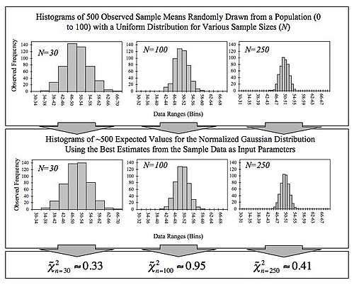
This figure demonstrates the central limit theorem. The sample means are generated using a random number generator, which draws numbers between 0 and 100 from a uniform probability distribution. It illustrates that increasing sample sizes result in the 500 measured sample means being more closely distributed about the population mean (50 in this case). It also compares the observed distributions with the distributions that would be expected for a normalized Gaussian distribution, and shows the chi-squared values that quantify the goodness of the fit (the fit is good if the reduced chi-squared value is less than or approximately equal to one). The input into the normalized Gaussian function is the mean of sample means (~50) and the mean sample standard deviation divided by the square root of the sample size (~28.87/√n), which is called the standard deviation of the mean (since it refers to the spread of sample means).
Another simulation using the binomial distribution. Random 0s and 1s were generated, and then their means calculated for sample sizes ranging from 1 to 2048. Note that as the sample size increases the tails become thinner and the distribution becomes more concentrated around the mean.
Regression
Regression analysis, and in particular ordinary least squares, specifies that a dependent variable depends according to some function upon one or more independent variables, with an additive error term. Various types of statistical inference on the regression assume that the error term is normally distributed. This assumption can be justified by assuming that the error term is actually the sum of many independent error terms; even if the individual error terms are not normally distributed, by the central limit theorem their sum can be well approximated by a normal distribution.
Given its importance to statistics, a number of papers and computer packages are available that demonstrate the convergence involved in the central limit theorem.[47]
The central limit theorem has an interesting history. The first version of this theorem was postulated by the French-born mathematician Abraham de Moivre who, in a remarkable article published in 1733, used the normal distribution to approximate the distribution of the number of heads resulting from many tosses of a fair coin. This finding was far ahead of its time, and was nearly forgotten until the famous French mathematician Pierre-Simon Laplace rescued it from obscurity in his monumental work Théorie analytique des probabilités, which was published in 1812. Laplace expanded De Moivre's finding by approximating the binomial distribution with the normal distribution. But as with De Moivre, Laplace's finding received little attention in his own time. It was not until the nineteenth century was at an end that the importance of the central limit theorem was discerned, when, in 1901, Russian mathematician Aleksandr Lyapunov defined it in general terms and proved precisely how it worked mathematically. Nowadays, the central limit theorem is considered to be the unofficial sovereign of probability theory.
I know of scarcely anything so apt to impress the imagination as the wonderful form of cosmic order expressed by the "Law of Frequency of Error". The law would have been personified by the Greeks and deified, if they had known of it. It reigns with serenity and in complete self-effacement, amidst the wildest confusion. The huger the mob, and the greater the apparent anarchy, the more perfect is its sway. It is the supreme law of Unreason. Whenever a large sample of chaotic elements are taken in hand and marshalled in the order of their magnitude, an unsuspected and most beautiful form of regularity proves to have been latent all along.
The actual term "central limit theorem" (in German: "zentraler Grenzwertsatz") was first used by George Pólya in 1920 in the title of a paper.[50][51] Pólya referred to the theorem as "central" due to its importance in probability theory. According to Le Cam, the French school of probability interprets the word central in the sense that "it describes the behaviour of the centre of the distribution as opposed to its tails".[51] The abstract of the paper On the central limit theorem of calculus of probability and the problem of moments by Pólya[50] in 1920 translates as follows.
The occurrence of the Gaussian probability density 1 = e−x2 in repeated experiments, in errors of measurements, which result in the combination of very many and very small elementary errors, in diffusion processes etc., can be explained, as is well-known, by the very same limit theorem, which plays a central role in the calculus of probability. The actual discoverer of this limit theorem is to be named Laplace; it is likely that its rigorous proof was first given by Tschebyscheff and its sharpest formulation can be found, as far as I am aware of, in an article by Liapounoff. ...
A thorough account of the theorem's history, detailing Laplace's foundational work, as well as Cauchy's, Bessel's and Poisson's contributions, is provided by Hald.[52] Two historical accounts, one covering the development from Laplace to Cauchy, the second the contributions by von Mises, Pólya, Lindeberg, Lévy, and Cramér during the 1920s, are given by Hans Fischer.[53] Le Cam describes a period around 1935.[51] Bernstein[54] presents a historical discussion focusing on the work of Pafnuty Chebyshev and his students Andrey Markov and Aleksandr Lyapunov that led to the first proofs of the CLT in a general setting.
A curious footnote to the history of the Central Limit Theorem is that a proof of a result similar to the 1922 Lindeberg CLT was the subject of Alan Turing's 1934 Fellowship Dissertation for King's College at the University of Cambridge. Only after submitting the work did Turing learn it had already been proved. Consequently, Turing's dissertation was not published.[55]
↑Bentkus, V. (2005). "A Lyapunov-type bound in ". Theory Probab. Appl. 49 (2): 311–323. doi:10.1137/S0040585X97981123.
↑Le Cam, L. (February 1986). "The Central Limit Theorem around 1935". Statistical Science. 1 (1): 78–91. JSTOR2245503.
↑Lévy, Paul (1937). Theorie de l'addition des variables aleatoires[Combination theory of unpredictable variables] (in French). Paris: Gauthier-Villars.
↑Gnedenko, Boris Vladimirovich; Kologorov, Andreĭ Nikolaevich; Doob, Joseph L.; Hsu, Pao-Lu (1968). Limit distributions for sums of independent random variables. Reading, MA: Addison-wesley.
↑Brewer, J. K. (1985). "Behavioral statistics textbooks: Source of myths and misconceptions?". Journal of Educational Statistics. 10 (3): 252–268. doi:10.3102/10769986010003252. S2CID119611584.
↑Yu, C.; Behrens, J.; Spencer, A. Identification of Misconception in the Central Limit Theorem and Related Concepts, American Educational Research Association lecture 19 April 1995
↑Rosenthal, Jeffrey Seth (2000). A First Look at Rigorous Probability Theory. World Scientific. Theorem 5.3.4, p. 47. ISBN981-02-4322-7.
↑Johnson, Oliver Thomas (2004). Information Theory and the Central Limit Theorem. Imperial College Press. p.88. ISBN1-86094-473-6.
↑Uchaikin, Vladimir V.; Zolotarev, V.M. (1999). Chance and Stability: Stable distributions and their applications. VSP. pp.61–62. ISBN90-6764-301-7.
↑Borodin, A. N.; Ibragimov, I. A.; Sudakov, V. N. (1995). Limit Theorems for Functionals of Random Walks. AMS Bookstore. Theorem 1.1, p. 8. ISBN0-8218-0438-3.
↑Hew, Patrick Chisan (2017). "Asymptotic distribution of rewards accumulated by alternating renewal processes". Statistics and Probability Letters. 129: 355–359. doi:10.1016/j.spl.2017.06.027.
↑Sunada, Toshikazu (2012). Topological Crystallography – With a View Towards Discrete Geometric Analysis. Surveys and Tutorials in the Applied Mathematical Sciences. Vol.6. Springer. ISBN978-4-431-54177-6.
↑Marasinghe, M.; Meeker, W.; Cook, D.; Shin, T. S. (August 1994). Using graphics and simulation to teach statistical concepts. Annual meeting of the American Statistician Association, Toronto, Canada.
↑Henk, Tijms (2004). Understanding Probability: Chance Rules in Everyday Life. Cambridge: Cambridge University Press. p.169. ISBN0-521-54036-4.
↑Bernstein, S. N. (1945). "On the work of P. L. Chebyshev in Probability Theory". In Bernstein., S. N. (ed.). Nauchnoe Nasledie P. L. Chebysheva. Vypusk Pervyi: Matematika[The Scientific Legacy of P. L. Chebyshev. Part I: Mathematics] (in Russian). Moscow & Leningrad: Academiya Nauk SSSR. p.174.
↑Zabell, S. L. (1995). "Alan Turing and the Central Limit Theorem". American Mathematical Monthly. 102 (6): 483–494. doi:10.1080/00029890.1995.12004608.
↑Jørgensen, Bent (1997). The Theory of Dispersion Models. Chapman & Hall. ISBN978-0412997112.
Klartag, Bo'az (2008). "A Berry–Esseen type inequality for convex bodies with an unconditional basis". Probability Theory and Related Fields. 145 (1–2): 1–33. arXiv:0705.0832. doi:10.1007/s00440-008-0158-6. S2CID10163322.
This page is based on this Wikipedia article Text is available under the CC BY-SA 4.0 license; additional terms may apply. Images, videos and audio are available under their respective licenses.