Factorial experiment

This article is about factorial design. For factor loadings, see Factor analysis. For factorial numbers (n!), see Factorial.

Designed experiments with full factorial design (left), response surface with second-degree polynomial (right)

In statistics, a full factorial experiment is an experiment whose design consists of two or more factors, each with discrete possible values or "levels", and whose experimental units take on all possible combinations of these levels across all such factors. A full factorial design may also be called a fully crossed design. Such an experiment allows the investigator to study the effect of each factor on the response variable, as well as the effects of interactions between factors on the response variable.

For the vast majority of factorial experiments, each factor has only two levels. For example, with two factors each taking two levels, a factorial experiment would have four treatment combinations in total, and is usually called a 2×2 factorial design. In such a design, the interaction between the variables is often the most important. This applies even to scenarios where a main effect and an interaction are present.

If the number of combinations in a full factorial design is too high to be logistically feasible, a fractional factorial design may be done, in which some of the possible combinations (usually at least half) are omitted.

Other terms for "treatment combinations" are often used, such as runs (of an experiment), points (viewing the combinations as vertices of a graph, and cells (arising as intersections of rows and columns).

History

Factorial designs were used in the 19th century by John Bennet Lawes and Joseph Henry Gilbert of the Rothamsted Experimental Station. ^[1]

Ronald Fisher argued in 1926 that "complex" designs (such as factorial designs) were more efficient than studying one factor at a time. ^[2] Fisher wrote,

"No aphorism is more frequently repeated in connection with field trials, than that we must ask Nature few questions, or, ideally, one question, at a time. The writer is convinced that this view is wholly mistaken."

Nature, he suggests, will best respond to "a logical and carefully thought out questionnaire". A factorial design allows the effect of several factors and even interactions between them to be determined with the same number of trials as are necessary to determine any one of the effects by itself with the same degree of accuracy.

Frank Yates made significant contributions, particularly in the analysis of designs, by the Yates analysis.

The term "factorial" may not have been used in print before 1935, when Fisher used it in his book The Design of Experiments . ^[3]

Advantages and disadvantages of factorial experiments

Many people examine the effect of only a single factor or variable. Compared to such one-factor-at-a-time (OFAT) experiments, factorial experiments offer several advantages ^{[4] [5]}

• Factorial designs are more efficient than OFAT experiments. They provide more information at similar or lower cost. They can find optimal conditions faster than OFAT experiments.
• When the effect of one factor is different for different levels of another factor, it cannot be detected by an OFAT experiment design. Factorial designs are required to detect such interactions. Use of OFAT when interactions are present can lead to serious misunderstanding of how the response changes with the factors.
• Factorial designs allow the effects of a factor to be estimated at several levels of the other factors, yielding conclusions that are valid over a range of experimental conditions.

The main disadvantage of the full factorial design is its sample size requirement, which grows exponentially with the number of factors or inputs considered. ^[6] Alternative strategies with improved computational efficiency include fractional factorial designs, Latin hypercube sampling, and quasi-random sampling techniques.

Example of advantages of factorial experiments

In his book, Improving Almost Anything: Ideas and Essays, statistician George Box gives many examples of the benefits of factorial experiments. Here is one. ^[7] Engineers at the bearing manufacturer SKF wanted to know if changing to a less expensive "cage" design would affect bearing life. The engineers asked Christer Hellstrand, a statistician, for help in designing the experiment. ^[8]

Box reports the following. "The results were assessed by an accelerated life test. … The runs were expensive because they needed to be made on an actual production line and the experimenters were planning to make four runs with the standard cage and four with the modified cage. Christer asked if there were other factors they would like to test. They said there were, but that making added runs would exceed their budget. Christer showed them how they could test two additional factors "for free" – without increasing the number of runs and without reducing the accuracy of their estimate of the cage effect. In this arrangement, called a 2×2×2 factorial design, each of the three factors would be run at two levels and all the eight possible combinations included. The various combinations can conveniently be shown as the vertices of a cube ... " "In each case, the standard condition is indicated by a minus sign and the modified condition by a plus sign. The factors changed were heat treatment, outer ring osculation, and cage design. The numbers show the relative lengths of lives of the bearings. If you look at [the cube plot], you can see that the choice of cage design did not make a lot of difference. … But, if you average the pairs of numbers for cage design, you get the [table below], which shows what the two other factors did. … It led to the extraordinary discovery that, in this particular application, the life of a bearing can be increased fivefold if the two factor(s) outer ring osculation and inner ring heat treatments are increased together."

Bearing life vs. heat and osculation

	Osculation −	Osculation +
Heat −	18	23
Heat +	21	106

"Remembering that bearings like this one have been made for decades, it is at first surprising that it could take so long to discover so important an improvement. A likely explanation is that, because most engineers have, until recently, employed only one factor at a time experimentation, interaction effects have been missed."

Example

The simplest factorial experiment contains two levels for each of two factors. Suppose an engineer wishes to study the total power used by each of two different motors, A and B, running at each of two different speeds, 2000 or 3000 RPM. The factorial experiment would consist of four experimental units: motor A at 2000 RPM, motor B at 2000 RPM, motor A at 3000 RPM, and motor B at 3000 RPM. Each combination of a single level selected from every factor is present once.

This experiment is an example of a 2² (or 2×2) factorial experiment, so named because it considers two levels (the base) for each of two factors (the power or superscript), or #levels^#factors, producing 2²=4 factorial points.

Cube plot for factorial design

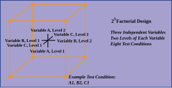
Designs can involve many independent variables. As a further example, the effects of three input variables can be evaluated in eight experimental conditions shown as the corners of a cube.

This can be conducted with or without replication, depending on its intended purpose and available resources. It will provide the effects of the three independent variables on the dependent variable and possible interactions.

Notation

Factorial experiments are described by two things: the number of factors, and the number of levels of each factor. For example, a 2×3 factorial experiment has two factors, the first at 2 levels and the second at 3 levels. Such an experiment has 2×3=6 treatment combinations or cells. Similarly, a 2×2×3 experiment has three factors, two at 2 levels and one at 3, for a total of 12 treatment combinations. If every factor has s levels (a so-called fixed-level or symmetric design), the experiment is typically denoted by s^k, where k is the number of factors. Thus a 2⁵ experiment has 5 factors, each at 2 levels. Experiments that are not fixed-level are said to be mixed-level or asymmetric.

There are various traditions to denote the levels of each factor. If a factor already has natural units, then those are used. For example, a shrimp aquaculture experiment ^[9] might have factors temperature at 25° and 35° centigrade, density at 80 or 160 shrimp/40 liters, and salinity at 10%, 25% and 40%. In many cases, though, the factor levels are simply categories, and the coding of levels is somewhat arbitrary. For example, the levels of an 6-level factor might simply be denoted 1, 2, ..., 6.

The cells in a 2 × 3 experiment

B A	1	2	3
1	11	12	13
2	21	22	23

Treatment combinations are denoted by ordered pairs or, more generally, ordered tuples. In the aquaculture experiment, the ordered triple (25, 80, 10) represents the treatment combination having the lowest level of each factor. In a general 2×3 experiment the ordered pair (2, 1) would indicate the cell in which factor A is at level 2 and factor B at level 1. The parentheses are often dropped, as shown in the accompanying table.

Cell notation in a 2×2 experiment

Both low	00	−−	(1)
A low	01	−+	a
B low	10	+−	b
Both high	11	++	ab

To denote factor levels in 2^k experiments, three particular systems appear in the literature:

• The values 1 and 0;
• the values 1 and −1, often simply abbreviated by + and −;
• A lower-case letter with the exponent 0 or 1.

If these values represent "low" and "high" settings of a treatment, then it is natural to have 1 represent "high", whether using 0 and 1 or −1 and 1. This is illustrated in the accompanying table for a 2×2 experiment. If the factor levels are simply categories, the correspondence might be different; for example, it is natural to represent "control" and "experimental" conditions by coding "control" as 0 if using 0 and 1, and as 1 if using 1 and −1. ^{[note 1]} An example of the latter is given below. That example illustrates another use of the coding +1 and −1.

For other fixed-level (s^k) experiments, the values 0, 1, ..., s−1 are often used to denote factor levels. These are the values of the integers modulo s when s is prime. ^{[note 2]}

Contrasts, main effects and interactions

Cell means in a 2 × 3 factorial experiment

B A	1	2	3
1	μ11	μ12	μ13
2	μ21	μ22	μ23

The expected response to a given treatment combination is called a cell mean, ^[11] usually denoted using the Greek letter μ. (The term cell is borrowed from its use in tables of data.) This notation is illustrated here for the 2 × 3 experiment.

A contrast in cell means is a linear combination of cell means in which the coefficients sum to 0. Contrasts are of interest in themselves, and are the building blocks by which main effects and interactions are defined.

In the 2 × 3 experiment illustrated here, the expression

${\displaystyle \mu _{11}-\mu _{12}}$

is a contrast that compares the mean responses of the treatment combinations 11 and 12. (The coefficients here are 1 and –1.) The contrast

${\displaystyle \mu _{11}+\mu _{12}+\mu _{13}-\mu _{21}-\mu _{22}-\mu _{23}}$

is said to belong to the main effect of factor A as it contrasts the responses to the "1" level of factor ${\displaystyle A}$ with those for the "2" level. The main effect of A is said to be absent if this expression equals 0.

Interaction in a factorial experiment is the lack of additivity between factors, and is also expressed by contrasts. In the 2 × 3 experiment, the contrasts

${\displaystyle \mu _{11}-\mu _{12}-\mu _{21}+\mu _{22}}$  and  ${\displaystyle \mu _{11}-\mu _{13}-\mu _{21}+\mu _{23}}$

belong to the A × B interaction; interaction is absent (additivity is present) if these expressions equal 0. ^{[12] [13]} . Additivity may be viewed as a kind of parallelism between factors, as illustrated in the Analysis section below.

Since it is the coefficients of these contrasts that carry the essential information, they are often displayed as column vectors. For the example above, such a table might look like this: ^[14]

Contrast vectors for the
2 × 3 factorial experiment

cell	${\displaystyle A}$	${\displaystyle B}$		${\displaystyle A\times B}$
11	1	1	0	1	1
12	1	−1	1	-1	0
13	1	0	−1	0	−1
21	−1	1	0	−1	-1
22	−1	−1	1	1	0
23	−1	0	−1	0	1

The columns of such a table are called contrast vectors: their components add up to 0. Each effect is determined by both the pattern of components in its columns and the number of columns.

The patterns of components of these columns reflect the general definitions given by Bose: ^[15]

• A contrast vector belongs to the main effect of a particular factor if the values of its components depend only on the level of that factor.

• A contrast vector belongs to the interaction of two factors, say A and B, if (i) the values of its components depend only on the levels of A and B, and (ii) it is orthogonal (perpendicular) to the contrast vectors representing the main effects of A and B. ^{[note 3]}

Similar definitions hold for interactions of more than two factors. In the 2 × 3 example, for instance, the pattern of the A column follows the pattern of the levels of factor A, indicated by the first component of each cell.

The number of columns needed to specify each effect is the degrees of freedom for the effect, ^{[note 4]} and is an essential quantity in the analysis of variance. The formula is as follows: ^{[17] [18]}

• A main effect for a factor with s levels has s−1 degrees of freedom.
• The interaction of two factors with s₁ and s₂ levels, respectively, has (s₁−1)(s₂−1) degrees of freedom.

The formula for more than two factors follows this pattern. In the 2 × 3 example above, the degrees of freedom for the two main effects and the interaction — the number of columns for each — are 1, 2 and 2, respectively.

Examples

In the tables in the following examples, the entries in the "cell" column are treatment combinations: The first component of each combination is the level of factor A, the second for factor B, and the third (in the 2 × 2 × 2 example) the level of factor C. The entries in each of the other columns sum to 0, so that each column is a contrast vector.

Contrast vectors in a ${\displaystyle 3\times 3}$ experiment

cell	${\displaystyle A}$		${\displaystyle B}$		${\displaystyle A\times B}$
00	1	1	1	1	1	1	1	1
01	1	1	-1	0	-1	0	-1	0
02	1	1	0	-1	0	-1	0	-1
10	-1	0	1	1	-1	-1	0	0
11	-1	0	-1	0	1	0	0	0
12	-1	0	0	-1	0	1	0	0
20	0	-1	1	1	0	0	-1	-1
21	0	-1	-1	0	0	0	1	0
22	0	-1	0	-1	0	0	0	1

A 3 × 3 experiment: Here we expect 3-1 = 2 degrees of freedom each for the main effects of factors A and B, and (3-1)(3-1) = 4 degrees of freedom for the A × B interaction. This accounts for the number of columns for each effect in the accompanying table.

The two contrast vectors for A depend only on the level of factor A. This can be seen by noting that the pattern of entries in each A column is the same as the pattern of the first component of "cell". (If necessary, sorting the table on A will show this.) Thus these two vectors belong to the main effect of A. Similarly, the two contrast vectors for B depend only on the level of factor B, namely the second component of "cell", so they belong to the main effect of B.

The last four column vectors belong to the A × B interaction, as their entries depend on the values of both factors, and as all four columns are orthogonal to the columns for A and B. The latter can be verified by taking dot products.

A 2 × 2 × 2 experiment: This will have 1 degree of freedom for every main effect and interaction. For example, a two-factor interaction will have (2-1)(2-1) = 1 degree of freedom. Thus just a single column is needed to specify each of the seven effects.

Contrast vectors in a ${\displaystyle 2\times 2\times 2}$ experiment

cell	${\displaystyle A}$	${\displaystyle B}$	${\displaystyle C}$	${\displaystyle AB}$	${\displaystyle AC}$	${\displaystyle BC}$	${\displaystyle ABC}$
000	1	1	1	1	1	1	1
001	1	1	−1	1	−1	−1	−1
010	1	−1	1	−1	1	−1	−1
011	1	−1	−1	−1	−1	1	1
100	−1	1	1	−1	−1	1	−1
101	−1	1	−1	−1	1	−1	1
110	−1	−1	1	1	−1	−1	1
111	−1	−1	−1	1	1	1	−1

The columns for A, B and C represent the corresponding main effects, as the entries in each column depend only on the level of the corresponding factor. For example, the entries in the B column follow the same pattern as the middle component of "cell", as can be seen by sorting on B.

The columns for AB, AC and BC represent the corresponding two-factor interactions. For example, (i) the entries in the BC column depend on the second and third (B and C) components of cell, and are independent of the first (A) component, as can be seen by sorting on BC; and (ii) the BC column is orthogonal to columns B and C, as can be verified by computing dot products.

Finally, the ABC column represents the three-factor interaction: its entries depend on the levels of all three factors, and it is orthogonal to the other six contrast vectors.

The first three columns of this table, read row-by-row, give an alternate representation of the eight treatment combinations: 000 corresponds to +++, 001 to ++−, etc.

In this table, the number 1 may be replaced by any constant, because the resulting columns will still be contrast vectors. It is common to use the number 1/4 in 2 × 2 × 2 experiments ^{[note 5]} to define each main effect or interaction, and to declare, for example, that the contrast

${\displaystyle (\mu _{000}+\mu _{001}+\mu _{010}+\mu _{011})/4-(\mu _{100}+\mu _{101}+\mu _{110}+\mu _{111})/4}$

is "the" main effect of factor A, a numerical quantity that can be estimated. ^[19]

Implementation

For more than two factors, a 2^k factorial experiment can usually be recursively designed from a 2^k−1 factorial experiment by replicating the 2^k−1 experiment, assigning the first replicate to the first (or low) level of the new factor, and the second replicate to the second (or high) level. This framework can be generalized to, e.g., designing three replicates for three level factors, etc.

A factorial experiment allows for estimation of experimental error in two ways. The experiment can be replicated, or the sparsity-of-effects principlecan often be exploited. Replication is more common for small experiments and is a very reliable way of assessing experimental error. When the number of factors is large (typically more than about 5 factors, but this does vary by application), replication of the design can become operationally difficult. In these cases, it is common to only run a single replicate of the design, and to assume that factor interactions of more than a certain order (say, between three or more factors) are negligible. Under this assumption, estimates of such high order interactions are estimates of an exact zero, thus really an estimate of experimental error.

When there are many factors, many experimental runs will be necessary, even without replication. For example, experimenting with 10 factors at two levels each produces 2¹⁰=1024 combinations. At some point this becomes infeasible due to high cost or insufficient resources. In this case, fractional factorial designs may be used.

As with any statistical experiment, the experimental runs in a factorial experiment should be randomized to reduce the impact that bias could have on the experimental results. In practice, this can be a large operational challenge.

Factorial experiments can be used when there are more than two levels of each factor. However, the number of experimental runs required for three-level (or more) factorial designs will be considerably greater than for their two-level counterparts. Factorial designs are therefore less attractive if a researcher wishes to consider more than two levels.

Analysis

Main article: Yates analysis

A factorial experiment can be analyzed using ANOVA or regression analysis. ^[20] To compute the main effect of a factor "A" in a 2-level experiment, subtract the average response of all experimental runs for which A was at its low (or first) level from the average response of all experimental runs for which A was at its high (or second) level.

Other useful exploratory analysis tools for factorial experiments include main effects plots, interaction plots, Pareto plots, and a normal probability plot of the estimated effects.

When the factors are continuous, two-level factorial designs assume that the effects are linear. If a quadratic effect is expected for a factor, a more complicated experiment should be used, such as a central composite design. Optimization of factors that could have quadratic effects is the primary goal of response surface methodology.

Analysis example

Montgomery ^[4] gives the following example of analysis of a factorial experiment:.

An engineer would like to increase the filtration rate (output) of a process to produce a chemical, and to reduce the amount of formaldehyde used in the process. Previous attempts to reduce the formaldehyde have lowered the filtration rate. The current filtration rate is 75 gallons per hour. Four factors are considered: temperature (A), pressure (B), formaldehyde concentration (C), and stirring rate (D). Each of the four factors will be tested at two levels.

Onwards, the minus (−) and plus (+) signs will indicate whether the factor is run at a low or high level, respectively.

Design matrix and resulting filtration rate

A	B	C	D	Filtration rate
−	−	−	−	45
+	−	−	−	71
−	+	−	−	48
+	+	−	−	65
−	−	+	−	68
+	−	+	−	60
−	+	+	−	80
+	+	+	−	65
−	−	−	+	43
+	−	−	+	100
−	+	−	+	45
+	+	−	+	104
−	−	+	+	75
+	−	+	+	86
−	+	+	+	70
+	+	+	+	96

• 
  Plot of the main effects showing the filtration rates for the low (−) and high (+) settings for each factor.
• 
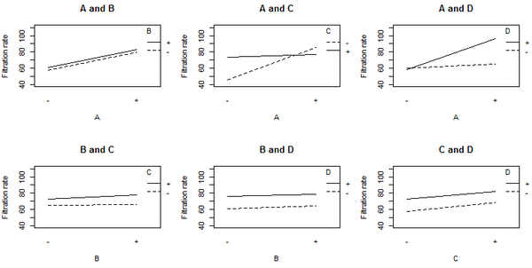
  Plot of the interaction effects showing the mean filtration rate at each of the four possible combinations of levels for a given pair of factors.

The non-parallel lines in the A:C interaction plot indicate that the effect of factor A depends on the level of factor C. A similar results holds for the A:D interaction. The graphs indicate that factor B has little effect on filtration rate. The analysis of variance (ANOVA) including all 4 factors and all possible interaction terms between them yields the coefficient estimates shown in the table below.

ANOVA results

Coefficients	Estimate
Intercept	70.063
A	10.813
B	1.563
C	4.938
D	7.313
A:B	0.063
A:C	−9.063
B:C	1.188
A:D	8.313
B:D	−0.188
C:D	−0.563
A:B:C	0.938
A:B:D	2.063
A:C:D	−0.813
B:C:D	−1.313
A:B:C:D	0.688

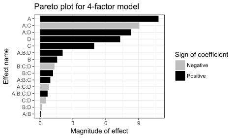
Pareto plot showing the relative magnitude of the factor coefficients.

Because there are 16 observations and 16 coefficients (intercept, main effects, and interactions), p-values cannot be calculated for this model. The coefficient values and the graphs suggest that the important factors are A, C, and D, and the interaction terms A:C and A:D.

The coefficients for A, C, and D are all positive in the ANOVA, which would suggest running the process with all three variables set to the high value. However, the main effect of each variable is the average over the levels of the other variables. The A:C interaction plot above shows that the effect of factor A depends on the level of factor C, and vice versa. Factor A (temperature) has very little effect on filtration rate when factor C is at the + level. But Factor A has a large effect on filtration rate when factor C (formaldehyde) is at the − level. The combination of A at the + level and C at the − level gives the highest filtration rate. This observation indicates how one-factor-at-a-time analyses can miss important interactions. Only by varying both factors A and C at the same time could the engineer discover that the effect of factor A depends on the level of factor C.

Cube plot for the ANOVA using factors A, C, and D, and the interaction terms A:C and A:D. The plot aids in visualizing the result and shows that the best combination is A+, D+, and C−.

The best filtration rate is seen when A and D are at the high level, and C is at the low level. This result also satisfies the objective of reducing formaldehyde (factor C). Because B does not appear to be important, it can be dropped from the model. Performing the ANOVA using factors A, C, and D, and the interaction terms A:C and A:D, gives the result shown in the following table, in which all the terms are significant (p-value < 0.05).

ANOVA results

Coefficient	Estimate	Standard error	t value	p-value
Intercept	70.062	1.104	63.444	2.3 × 10−14
A	10.812	1.104	9.791	1.9 × 10−6
C	4.938	1.104	4.471	1.2 × 10−3
D	7.313	1.104	6.622	5.9 × 10−5
A:C	−9.063	1.104	−8.206	9.4 × 10−6
A:D	8.312	1.104	7.527	2 × 10−5

See also

• Combinatorial design
• Design of experiments
• Orthogonal array
• Plackett–Burman design
• Taguchi methods
• Welch's t-test

Explanatory footnotes

1. This choice gives the correspondence 01 ←→ +−, the opposite of that given in the table. There are also algebraic reasons for doing this. The choice of coding via + and − is not important "as long as the labeling is consistent." ^[10]
2. This choice of factor levels facilitates the use of algebra to handle certain issues of experimental design. If s is a power of a prime, the levels may be denoted by the elements of the finite field GF(s) for the same reason.
3. Orthogonality is determined by computing the dot product of vectors.
4. The degrees of freedom for an effect is actually the dimension of a vector space, namely the space of all contrast vectors belonging to that effect. ^[16]
5. And 1/2^k-1 in 2^k experiments.

Notes

1. Yates, Frank; Mather, Kenneth (1963). "Ronald Aylmer Fisher". Biographical Memoirs of Fellows of the Royal Society . London, England: Royal Society. 9: 91–120. doi: 10.1098/rsbm.1963.0006 .
2. Fisher, Ronald (1926). "The Arrangement of Field Experiments" (PDF). Journal of the Ministry of Agriculture of Great Britain . London, England: Ministry of Agriculture and Fisheries. 33: 503–513.
3. "Earliest Known Uses of Some of the Words of Mathematics (F)". jeff560.tripod.com.
4. Montgomery, Douglas C. (2013). Design and Analysis of Experiments (8th ed.). Hoboken, New Jersey: Wiley. ISBN   978-1-119-32093-7.
5. Oehlert, Gary (2000). A First Course in Design and Analysis of Experiments (Revised ed.). New York City: W. H. Freeman and Company. ISBN   978-0-7167-3510-6.
6. Tong, C. (2006). "Refinement strategies for stratified sampling methods". Reliability Engineering & System Safety. 91 (10–11): 1257–1265. doi:10.1016/j.ress.2005.11.027.
7. George E.P., Box (2006). Improving Almost Anything: Ideas and Essays (Revised ed.). Hoboken, New Jersey: Wiley. ASIN   B01FKSM9VY.
8. Hellstrand, C.; Oosterhoorn, A. D.; Sherwin, D. J.; Gerson, M. (24 February 1989). "The Necessity of Modern Quality Improvement and Some Experience with its Implementation in the Manufacture of Rolling Bearings [and Discussion]". Philosophical Transactions of the Royal Society. 327 (1596): 529–537. doi:10.1098/rsta.1989.0008. S2CID   122252479.
9. Kuehl (2000 , pp. 200–205)
10. Box, Hunter & Hunter (1978, p. 307)
11. Hocking (1985 , p. 73). Hocking and others use the term "population mean" for expected value.
12. Graybill (1976 , p. 559-560)
13. Beder (2022 , pp. 29–30)
14. Beder (2022 , Example 5.21)
15. Bose (1947 , pp. 110–111)
16. Cheng (2019, p. 77)
17. Kuehl (2000 , p. 202)
18. Cheng (2019 , p. 78)
19. Box, Hunter & Hunter (1978 , p. 311)
20. Cohen, J (1968). "Multiple regression as a general data-analytic system". Psychological Bulletin. 70 (6): 426–443. CiteSeerX   10.1.1.476.6180 . doi:10.1037/h0026714.

References

• Beder, Jay H. (2022). Linear Models and Design. Cham, Switzerland: Springer. doi:10.1007/978-3-031-08176-7. ISBN   978-3-031-08175-0. S2CID   253542415.
• Bose, R. C. (1947). "Mathematical theory of the symmetrical factorial design". Sankhya. 8: 107–166.
• Box, G. E.; Hunter, W. G.; Hunter, J. S. (1978). Statistics for Experimenters: An Introduction to Design, Data Analysis and Model Building. Wiley. ISBN   978-0-471-09315-2.
• Box, G. E.; Hunter, W. G.; Hunter, J. S. (2005). Statistics for Experimenters: Design, Innovation, and Discovery (2nd ed.). Wiley. ISBN   978-0-471-71813-0.
• Cheng, Ching-Shui (2019). Theory of Factorial Design: Single- and Multi-Stratum Experiments. Boca Raton, Florida: CRC Press. ISBN   978-0-367-37898-1.
• Dean, Angela; Voss, Daniel; Draguljić, Danel (2017). Design and Analysis of Experiments (2nd ed.). Cham, Switzerland: Springer. ISBN   978-3-319-52250-0.
• Graybill, Franklin A. (1976). Fundamental Concepts in the Design of Experiments (3rd ed.). New York: Holt, Rinehart and Winston. ISBN   0-03-061706-5.
• Hicks, Charles R. (1982). Theory and Application of the Linear Model. Pacific Grove, CA: Wadsworth & Brooks/Cole. ISBN   0-87872-108-8.
• Hocking, Ronald R. (1985). The Analysis of Linear Models. Pacific Grove, CA: Brooks/Cole. ISBN   978-0534036188.
• Kuehl, Robert O. (2000). Design of Experiments: Statistical Principles of Research Design and Analysis (2nd ed.). Pacific Grove,CA: Brooks/Cole. ISBN   978-0534368340.
• Wu, C. F. Jeff; Hamada, Michael S. (30 March 2021). Experiments: Planning, Analysis, and Optimization. John Wiley & Sons. ISBN   978-1-119-47010-6.

External links

• Factorial Designs (California State University, Fresno)
• GOV.UK Factorial randomised controlled trials (Public Health England)