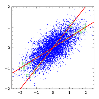
Ridge regression is a method of estimating the coefficients of multiple-regression models in scenarios where the independent variables are highly correlated. It has been used in many fields including econometrics, chemistry, and engineering. Also known as Tikhonov regularization, named for Andrey Tikhonov, it is a method of regularization of ill-posed problems. It is particularly useful to mitigate the problem of multicollinearity in linear regression, which commonly occurs in models with large numbers of parameters. In general, the method provides improved efficiency in parameter estimation problems in exchange for a tolerable amount of bias.
In statistics, and particularly in econometrics, the reduced form of a system of equations is the result of solving the system for the endogenous variables. This gives the latter as functions of the exogenous variables, if any. In econometrics, the equations of a structural form model are estimated in their theoretically given form, while an alternative approach to estimation is to first solve the theoretical equations for the endogenous variables to obtain reduced form equations, and then to estimate the reduced form equations.
In statistics, econometrics, epidemiology and related disciplines, the method of instrumental variables (IV) is used to estimate causal relationships when controlled experiments are not feasible or when a treatment is not successfully delivered to every unit in a randomized experiment. Intuitively, IVs are used when an explanatory variable of interest is correlated with the error term (endogenous), in which case ordinary least squares and ANOVA give biased results. A valid instrument induces changes in the explanatory variable but has no independent effect on the dependent variable and is not correlated with the error term, allowing a researcher to uncover the causal effect of the explanatory variable on the dependent variable.
In statistics, omitted-variable bias (OVB) occurs when a statistical model leaves out one or more relevant variables. The bias results in the model attributing the effect of the missing variables to those that were included.
In statistics, the theory of minimum norm quadratic unbiased estimation (MINQUE) was developed by C. R. Rao. MINQUE is a theory alongside other estimation methods in estimation theory, such as the method of moments or maximum likelihood estimation. Similar to the theory of best linear unbiased estimation, MINQUE is specifically concerned with linear regression models. The method was originally conceived to estimate heteroscedastic error variance in multiple linear regression. MINQUE estimators also provide an alternative to maximum likelihood estimators or restricted maximum likelihood estimators for variance components in mixed effects models. MINQUE estimators are quadratic forms of the response variable and are used to estimate a linear function of the variances.

In statistics, ordinary least squares (OLS) is a type of linear least squares method for choosing the unknown parameters in a linear regression model by the principle of least squares: minimizing the sum of the squares of the differences between the observed dependent variable in the input dataset and the output of the (linear) function of the independent variable. Some sources consider OLS to be linear regression.
In econometrics, endogeneity broadly refers to situations in which an explanatory variable is correlated with the error term. The distinction between endogenous and exogenous variables originated in simultaneous equations models, where one separates variables whose values are determined by the model from variables which are predetermined. Ignoring simultaneity in the estimation leads to biased estimates as it violates the exogeneity assumption of the Gauss–Markov theorem. The problem of endogeneity is often ignored by researchers conducting non-experimental research and doing so precludes making policy recommendations. Instrumental variable techniques are commonly used to mitigate this problem.
Vector autoregression (VAR) is a statistical model used to capture the relationship between multiple quantities as they change over time. VAR is a type of stochastic process model. VAR models generalize the single-variable (univariate) autoregressive model by allowing for multivariate time series. VAR models are often used in economics and the natural sciences.
In econometrics, the seemingly unrelated regressions (SUR) or seemingly unrelated regression equations (SURE) model, proposed by Arnold Zellner in (1962), is a generalization of a linear regression model that consists of several regression equations, each having its own dependent variable and potentially different sets of exogenous explanatory variables. Each equation is a valid linear regression on its own and can be estimated separately, which is why the system is called seemingly unrelated, although some authors suggest that the term seemingly related would be more appropriate, since the error terms are assumed to be correlated across the equations.
In statistics, a tobit model is any of a class of regression models in which the observed range of the dependent variable is censored in some way. The term was coined by Arthur Goldberger in reference to James Tobin, who developed the model in 1958 to mitigate the problem of zero-inflated data for observations of household expenditure on durable goods. Because Tobin's method can be easily extended to handle truncated and other non-randomly selected samples, some authors adopt a broader definition of the tobit model that includes these cases.
In statistics, a fixed effects model is a statistical model in which the model parameters are fixed or non-random quantities. This is in contrast to random effects models and mixed models in which all or some of the model parameters are random variables. In many applications including econometrics and biostatistics a fixed effects model refers to a regression model in which the group means are fixed (non-random) as opposed to a random effects model in which the group means are a random sample from a population. Generally, data can be grouped according to several observed factors. The group means could be modeled as fixed or random effects for each grouping. In a fixed effects model each group mean is a group-specific fixed quantity.
In statistics, semiparametric regression includes regression models that combine parametric and nonparametric models. They are often used in situations where the fully nonparametric model may not perform well or when the researcher wants to use a parametric model but the functional form with respect to a subset of the regressors or the density of the errors is not known. Semiparametric regression models are a particular type of semiparametric modelling and, since semiparametric models contain a parametric component, they rely on parametric assumptions and may be misspecified and inconsistent, just like a fully parametric model.
In statistics, the multivariate t-distribution is a multivariate probability distribution. It is a generalization to random vectors of the Student's t-distribution, which is a distribution applicable to univariate random variables. While the case of a random matrix could be treated within this structure, the matrix t-distribution is distinct and makes particular use of the matrix structure.
The Heckman correction is a statistical technique to correct bias from non-randomly selected samples or otherwise incidentally truncated dependent variables, a pervasive issue in quantitative social sciences when using observational data. Conceptually, this is achieved by explicitly modelling the individual sampling probability of each observation together with the conditional expectation of the dependent variable. The resulting likelihood function is mathematically similar to the tobit model for censored dependent variables, a connection first drawn by James Heckman in 1974. Heckman also developed a two-step control function approach to estimate this model, which avoids the computational burden of having to estimate both equations jointly, albeit at the cost of inefficiency. Heckman received the Nobel Memorial Prize in Economic Sciences in 2000 for his work in this field.
An error correction model (ECM) belongs to a category of multiple time series models most commonly used for data where the underlying variables have a long-run common stochastic trend, also known as cointegration. ECMs are a theoretically-driven approach useful for estimating both short-term and long-term effects of one time series on another. The term error-correction relates to the fact that last-period's deviation from a long-run equilibrium, the error, influences its short-run dynamics. Thus ECMs directly estimate the speed at which a dependent variable returns to equilibrium after a change in other variables.

In statistics, an errors-in-variables model or a measurement error model is a regression model that accounts for measurement errors in the independent variables. In contrast, standard regression models assume that those regressors have been measured exactly, or observed without error; as such, those models account only for errors in the dependent variables, or responses.
In econometrics, the Arellano–Bond estimator is a generalized method of moments estimator used to estimate dynamic models of panel data. It was proposed in 1991 by Manuel Arellano and Stephen Bond, based on the earlier work by Alok Bhargava and John Denis Sargan in 1983, for addressing certain endogeneity problems. The GMM-SYS estimator is a system that contains both the levels and the first difference equations. It provides an alternative to the standard first difference GMM estimator.
Control functions are statistical methods to correct for endogeneity problems by modelling the endogeneity in the error term. The approach thereby differs in important ways from other models that try to account for the same econometric problem. Instrumental variables, for example, attempt to model the endogenous variable X as an often invertible model with respect to a relevant and exogenous instrument Z. Panel analysis uses special data properties to difference out unobserved heterogeneity that is assumed to be fixed over time.
In least squares estimation problems, sometimes one or more regressors specified in the model are not observable. One way to circumvent this issue is to estimate or generate regressors from observable data. This generated regressor method is also applicable to unobserved instrumental variables. Under some regularity conditions, consistency and asymptotic normality of least squares estimator is preserved, but asymptotic variance has a different form in general.
In statistics and econometrics, optimal instruments are a technique for improving the efficiency of estimators in conditional moment models, a class of semiparametric models that generate conditional expectation functions. To estimate parameters of a conditional moment model, the statistician can derive an expectation function and use the generalized method of moments (GMM). However, there are infinitely many moment conditions that can be generated from a single model; optimal instruments provide the most efficient moment conditions.


