Economic equilibrium

Last updated
Economic equilibrium
A solution concept in game theory
Relationship
Subset of Equilibrium, Free market
Superset of Competitive equilibrium, Nash equilibrium, Intertemporal equilibrium, Recursive competitive equilibrium
Significance
Used formostly Perfect competition, but also some Imperfect competition

In economics, economic equilibrium is a situation in which economic forces such as supply and demand are balanced and in the absence of external influences the (equilibrium) values of economic variables will not change. For example, in the standard text perfect competition, equilibrium occurs at the point at which quantity demanded and quantity supplied are equal. [1]

Contents

Market equilibrium in this case is a condition where a market price is established through competition such that the amount of goods or services sought by buyers is equal to the amount of goods or services produced by sellers. This price is often called the competitive price or market clearing price and will tend not to change unless demand or supply changes, and quantity is called the "competitive quantity" or market clearing quantity. But the concept of equilibrium in economics also applies to imperfectly competitive markets, where it takes the form of a Nash equilibrium.

Understanding economic equilibrium

An economic equilibrium is a situation when the economic agent cannot change the situation by adopting any strategy. The concept has been borrowed from the physical sciences. Take a system where physical forces are balanced for instance.This economically interpreted means no further change ensues.

Properties of equilibrium

Three basic properties of equilibrium in general have been proposed by Huw Dixon. [2] These are:

Example: competitive equilibrium

Competitive Equilibrium: Price equates supply and demand.
P - price
Q - quantity demanded and supplied
S - supply curve
D - demand curve
P0 - equilibrium price
A - excess demand - when P<P0
B - excess supply - when P>P0 Price of market balance.gif
Competitive Equilibrium: Price equates supply and demand.
  • P – price
  • Q – quantity demanded and supplied
  • S – supply curve
  • D – demand curve
  • P0 – equilibrium price
  • A – excess demand – when P<P0
  • B – excess supply – when P>P0

In a competitive equilibrium, supply equals demand. Property P1 is satisfied, because at the equilibrium price the amount supplied is equal to the amount demanded. Property P2 is also satisfied. Demand is chosen to maximize utility given the market price: no one on the demand side has any incentive to demand more or less at the prevailing price. Likewise supply is determined by firms maximizing their profits at the market price: no firm will want to supply any more or less at the equilibrium price. Hence, agents on neither the demand side nor the supply side will have any incentive to alter their actions.

To see whether Property P3 is satisfied, consider what happens when the price is above the equilibrium. In this case there is an excess supply, with the quantity supplied exceeding that demanded. This will tend to put downward pressure on the price to make it return to equilibrium. Likewise where the price is below the equilibrium point (also known as the "sweet spot" [3] ) there is a shortage in supply leading to an increase in prices back to equilibrium. Not all equilibria are "stable" in the sense of equilibrium property P3. It is possible to have competitive equilibria that are unstable. However, if an equilibrium is unstable, it raises the question of reaching it. Even if it satisfies properties P1 and P2, the absence of P3 means that the market can only be in the unstable equilibrium if it starts off there.

In most simple microeconomic stories of supply and demand a static equilibrium is observed in a market; however, economic equilibrium can be also dynamic. Equilibrium may also be economy-wide or general, as opposed to the partial equilibrium of a single market. Equilibrium can change if there is a change in demand or supply conditions. For example, an increase in supply will disrupt the equilibrium, leading to lower prices. Eventually, a new equilibrium will be attained in most markets. Then, there will be no change in price or the amount of output bought and sold — until there is an exogenous shift in supply or demand (such as changes in technology or tastes). That is, there are no endogenous forces leading to the price or the quantity.

Example: monopolist equilibrium

In a monopoly, marginal revenue (MR) equals marginal cost (MC). The equilibrium quantity is obtained from where MR and MC intersect and the equilibrium price can be found on the demand curve where MR = MC. Property P1 is not satisfied because the amount demand and the amount supplied at the equilibrium price are not equal. Property P2 is not satisfied. Because the monopolist's profit-maximizing quantity is different from the socially-maximizing quantity, consumer's have an incentive to demand more at the equilibrium price. However, at the market price, monopolists maximize their profits so they have no incentive to change their price. Therefore, agents on the demand side have an incentive to alter their actions while the agents on the supply side do not have any incentive to alter their actions.

In order to determine if Property P3 is satisfied, the same situations used to determine P3 in a competitive equilibrium can be used. When there is an excess in supply, monopolists will realize that the equilibrium is not at the profit-maximizing quantity and will put upward pressure on the price to make it return to equilibrium. This is the same case when the price is above the equilibrium and the shortage in supply leads the monopolist to decrease the supply to return to the profit-maximizing quantity. Therefore the equilibrium is the result of stability.

Example: Nash equilibrium

Equilibrium quantities as a solution to two reaction functions in Cournot duopoly. Firm 1's reaction function q1=R1(q2) gives its optimal output q1 to a given output q2 of firm 2. Likewise, firm 2's reaction function q2=R2(q1). The Cournot-Nash equilibrium occurs where the two reaction functions intersect and both firms are choosing the optimal output given the output of the other firm. Economics cournot diag4 svg.svg
Equilibrium quantities as a solution to two reaction functions in Cournot duopoly. Firm 1's reaction function q1=R1(q2) gives its optimal output q1 to a given output q2 of firm 2. Likewise, firm 2's reaction function q2=R2(q1). The Cournot-Nash equilibrium occurs where the two reaction functions intersect and both firms are choosing the optimal output given the output of the other firm.

The Nash equilibrium is widely used in economics as the main alternative to competitive equilibrium. It is used whenever there is a strategic element to the behavior of agents and the "price taking" assumption of competitive equilibrium is inappropriate. The first use of the Nash equilibrium was in the Cournot duopoly as developed by Antoine Augustin Cournot in his 1838 book. [4] Both firms produce a homogenous product: given the total amount supplied by the two firms, the (single) industry price is determined using the demand curve. This determines the revenues of each firm (the industry price times the quantity supplied by the firm). The profit of each firm is then this revenue minus the cost of producing the output. Clearly, there is a strategic interdependence between the two firms. If one firm varies its output, this will in turn affect the market price and so the revenue and profits of the other firm. We can define the payoff function which gives the profit of each firm as a function of the two outputs chosen by the firms. Cournot assumed that each firm chooses its own output to maximize its profits given the output of the other firm. The Nash equilibrium occurs when both firms are producing the outputs which maximize their own profit given the output of the other firm.

In terms of the equilibrium properties, we can see that P2 is satisfied: in a Nash equilibrium, neither firm has an incentive to deviate from the Nash equilibrium given the output of the other firm. P1 is satisfied since the payoff function ensures that the market price is consistent with the outputs supplied and that each firms profits equal revenue minus cost at this output.

Is the equilibrium stable as required by P3? Cournot himself argued that it was stable using the stability concept implied by best response dynamics. The reaction function for each firm gives the output which maximizes profits (best response) in terms of output for a firm in terms of a given output of the other firm. In the standard Cournot model this is downward sloping: if the other firm produces a higher output, the best response involves producing less. Best response dynamics involves firms starting from some arbitrary position and then adjusting output to their best-response to the previous output of the other firm. So long as the reaction functions have a slope of less than -1, this will converge to the Nash equilibrium. However, this stability story is open to much criticism. As Dixon argues: "The crucial weakness is that, at each step, the firms behave myopically: they choose their output to maximize their current profits given the output of the other firm, but ignore the fact that the process specifies that the other firm will adjust its output...". [5] There are other concepts of stability that have been put forward for the Nash equilibrium, evolutionary stability for example.

Market clearing prices

Most economists, for example Paul Samuelson, [6] caution against attaching a normative meaning (value judgement) to the equilibrium price. For example, food markets may be in equilibrium at the same time that people are starving (because they cannot afford to pay the high equilibrium price).

Indeed, this occurred during the Great Famine in Ireland in 1845–52, where food was exported though people were starving, due to the greater profits in selling to the English – the equilibrium price of the Irish-British market for potatoes was above the price that Irish farmers could afford, and thus (among other reasons) they starved. [7]

Interpretations

In most interpretations, classical economists such as Adam Smith maintained that the free market would tend towards economic equilibrium through the price mechanism. That is, any excess supply (market surplus or glut) would lead to price cuts, which decrease the quantity supplied (by reducing the incentive to produce and sell the product) and increase the quantity demanded (by offering consumers bargains), automatically abolishing the glut. Similarly, in an unfettered market, any excess demand (or shortage) would lead to price increases, reducing the quantity demanded (as customers are priced out of the market) and increasing in the quantity supplied (as the incentive to produce and sell a product rises). As before, the disequilibrium (here, the shortage) disappears. This automatic abolition of non-market-clearing situations distinguishes markets from central planning schemes, which often have a difficult time getting prices right and suffer from persistent shortages of goods and services. [8]

This view came under attack from at least two viewpoints. Modern mainstream economics points to cases where equilibrium does not correspond to market clearing (but instead to unemployment), as with the efficiency wage hypothesis in labor economics. In some ways parallel is the phenomenon of credit rationing, in which banks hold interest rates low to create an excess demand for loans, so they can pick and choose whom to lend to. Further, economic equilibrium can correspond with monopoly, where the monopolistic firm maintains an artificial shortage to prop up prices and to maximize profits. Finally, Keynesian macroeconomics points to underemployment equilibrium, where a surplus of labor (i.e., cyclical unemployment) co-exists for a long time with a shortage of aggregate demand.

Solving for the competitive equilibrium price

To find the equilibrium price, one must either plot the supply and demand curves, or solve for the expressions for supply and demand being equal.

An example may be:

Simple supply and demand.svg

In the diagram, depicting simple set of supply and demand curves, the quantity demanded and supplied at price P are equal.

At any price above P supply exceeds demand, while at a price below P the quantity demanded exceeds that supplied. In other words, prices where demand and supply are out of balance are termed points of disequilibrium, creating shortages and oversupply. Changes in the conditions of demand or supply will shift the demand or supply curves. This will cause changes in the equilibrium price and quantity in the market.

Consider the following demand and supply schedule:

Price ($)DemandSupply
8.006,00018,000
7.008,00016,000
6.0010,00014,000
5.0012,00012,000
4.0014,00010,000
3.0016,0008,000
2.0018,0006,000
1.0020,0004,000

When there is a shortage in the market we see that, to correct this disequilibrium, the price of the good will be increased back to a price of $5.00, thus lessening the quantity demanded and increasing the quantity supplied thus that the market is in balance.

When there is an oversupply of a good, such as when price is above $6.00, then we see that producers will decrease the price to increase the quantity demanded for the good, thus eliminating the excess and taking the market back to equilibrium.

Influences changing price

A change in equilibrium price may occur through a change in either the supply or demand schedules. For instance, starting from the above supply-demand configuration, an increased level of disposable income may produce a new demand schedule, such as the following:

Price ($)DemandSupply
8.0010,00018,000
7.0012,00016,000
6.0014,00014,000
5.0016,00012,000
4.0018,00010,000
3.0020,0008,000
2.0022,0006,000
1.0024,0004,000

Here we see that an increase in disposable income would increase the quantity demanded of the good by 2,000 units at each price. This increase in demand would have the effect of shifting the demand curve rightward. The result is a change in the price at which quantity supplied equals quantity demanded. In this case we see that the two now equal each other at an increased price of $6.00. A decrease in disposable income would have the exact opposite effect on the market equilibrium.

We will also see similar behaviour in price when there is a change in the supply schedule, occurring through technological changes, or through changes in business costs. An increase in technological usage or know-how or a decrease in costs would have the effect of increasing the quantity supplied at each price, thus reducing the equilibrium price. On the other hand, a decrease in technology or increase in business costs will decrease the quantity supplied at each price, thus increasing equilibrium price.

The process of comparing two static equilibria to each other, as in the above example, is known as comparative statics. For example, since a rise in consumers' income leads to a higher price (and a decline in consumers' income leads to a fall in the price — in each case the two things change in the same direction), we say that the comparative static effect of consumer income on the price is positive. This is another way of saying that the total derivative of price with respect to consumer income is greater than zero.

Dynamic equilibrium

Whereas in a static equilibrium all quantities have unchanging values, in a dynamic equilibrium various quantities may all be growing at the same rate, leaving their ratios unchanging. For example, in the neoclassical growth model, the working population is growing at a rate which is exogenous (determined outside the model, by non-economic forces). In dynamic equilibrium, output and the physical capital stock also grow at that same rate, with output per worker and the capital stock per worker unchanging. Similarly, in models of inflation a dynamic equilibrium would involve the price level, the nominal money supply, nominal wage rates, and all other nominal values growing at a single common rate, while all real values are unchanging, as is the inflation rate. [9]

The process of comparing two dynamic equilibria to each other is known as comparative dynamics. For example, in the neoclassical growth model, starting from one dynamic equilibrium based in part on one particular saving rate, a permanent increase in the saving rate leads to a new dynamic equilibrium in which there are permanently higher capital per worker and productivity per worker, but an unchanged growth rate of output; so it is said that in this model the comparative dynamic effect of the saving rate on capital per worker is positive but the comparative dynamic effect of the saving rate on the output growth rate is zero.

Disequilibrium

Disequilibrium characterizes a market that is not in equilibrium. [10] Disequilibrium can occur extremely briefly or over an extended period of time. At the other extreme, many economists view labor markets as being in a state of disequilibriumspecifically one of excess supplyover extended periods of time. Goods markets are somewhere in between: prices of some goods, while sluggish in adjusting due to menu costs, long-term contracts, and other impediments, do not stay at disequilibrium levels indefinitely.

See also

Related Research Articles

A duopoly is a type of oligopoly where two firms have dominant or exclusive control over a market, and most of the competition within that market occurs directly between them.

<span class="mw-page-title-main">Microeconomics</span> Behavior of individuals and firms

Microeconomics is a branch of economics that studies the behavior of individuals and firms in making decisions regarding the allocation of scarce resources and the interactions among these individuals and firms. Microeconomics focuses on the study of individual markets, sectors, or industries as opposed to the national economy as a whole, which is studied in macroeconomics.

An oligopoly is a market in which control over an industry lies in the hands of a few large sellers who own a dominant share of the market. Oligopolistic markets have homogenous products, few market participants, and inelastic demand for the products in those industries. As a result of their significant market power, firms in oligopolistic markets can influence prices through manipulating the supply function. Firms in an oligopoly are also mutually interdependent, as any action by one firm is expected to affect other firms in the market and evoke a reaction or consequential action. As a result, firms in oligopolistic markets often resort to collusion as means of maximising profits.

In economics, specifically general equilibrium theory, a perfect market, also known as an atomistic market, is defined by several idealizing conditions, collectively called perfect competition, or atomistic competition. In theoretical models where conditions of perfect competition hold, it has been demonstrated that a market will reach an equilibrium in which the quantity supplied for every product or service, including labor, equals the quantity demanded at the current price. This equilibrium would be a Pareto optimum.

<span class="mw-page-title-main">Supply and demand</span> Economic model of price determination in a market

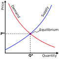
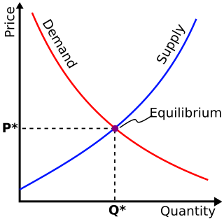
In microeconomics, supply and demand is an economic model of price determination in a market. It postulates that, holding all else equal, in a competitive market, the unit price for a particular good, or other traded item such as labor or current financial assets, will vary until it settles at a point where the quantity demanded will equal the quantity supplied, resulting in an economic equilibrium for price and quantity transacted. The concept of supply and demand forms the theoretical basis of modern economics.

This aims to be a complete article list of economics topics:

<span class="mw-page-title-main">Profit maximization</span> Process to determine the highest profits for a firm

In economics, profit maximization is the short run or long run process by which a firm may determine the price, input and output levels that will lead to the highest possible total profit. In neoclassical economics, which is currently the mainstream approach to microeconomics, the firm is assumed to be a "rational agent" which wants to maximize its total profit, which is the difference between its total revenue and its total cost.

In economics, effective demand (ED) in a market is the demand for a product or service which occurs when purchasers are constrained in a different market. It contrasts with notional demand, which is the demand that occurs when purchasers are not constrained in any other market. In the aggregated market for goods in general, demand, notional or effective, is referred to as aggregate demand. The concept of effective supply parallels the concept of effective demand. The concept of effective demand or supply becomes relevant when markets do not continuously maintain equilibrium prices.

In economics, quantity adjustment is the process by which a market surplus leads to a cut-back in the quantity supplied or a market shortage causes an increase in supplied quantity. It is one possible result of supply and demand disequilibrium in a market. Quantity adjustment is complementary to pricing.

<span class="mw-page-title-main">Market clearing</span>

In economics, market clearing is the process by which, in an economic market, the supply of whatever is traded is equated to the demand so that there is no excess supply or demand, ensuring that there is neither a surplus nor a shortage. The new classical economics assumes that in any given market, assuming that all buyers and sellers have access to information and that there is no "friction" impeding price changes, prices constantly adjust up or down to ensure market clearing.

<span class="mw-page-title-main">Marginal revenue</span> Additional total revenue generated by increasing product sales by 1 unit

Marginal revenue is a central concept in microeconomics that describes the additional total revenue generated by increasing product sales by 1 unit. Marginal revenue is the increase in revenue from the sale of one additional unit of product, i.e., the revenue from the sale of the last unit of product. It can be positive or negative. Marginal revenue is an important concept in vendor analysis. To derive the value of marginal revenue, it is required to examine the difference between the aggregate benefits a firm received from the quantity of a good and service produced last period and the current period with one extra unit increase in the rate of production. Marginal revenue is a fundamental tool for economic decision making within a firm's setting, together with marginal cost to be considered.

Bertrand competition is a model of competition used in economics, named after Joseph Louis François Bertrand (1822–1900). It describes interactions among firms (sellers) that set prices and their customers (buyers) that choose quantities at the prices set. The model was formulated in 1883 by Bertrand in a review of Antoine Augustin Cournot's book Recherches sur les Principes Mathématiques de la Théorie des Richesses (1838) in which Cournot had put forward the Cournot model. Cournot's model argued that each firm should maximise its profit by selecting a quantity level and then adjusting price level to sell that quantity. The outcome of the model equilibrium involved firms pricing above marginal cost; hence, the competitive price. In his review, Bertrand argued that each firm should instead maximise its profits by selecting a price level that undercuts its competitors' prices, when their prices exceed marginal cost. The model was not formalized by Bertrand; however, the idea was developed into a mathematical model by Francis Ysidro Edgeworth in 1889.

Cournot competition is an economic model used to describe an industry structure in which companies compete on the amount of output they will produce, which they decide on independently of each other and at the same time. It is named after Antoine Augustin Cournot (1801–1877) who was inspired by observing competition in a spring water duopoly. It has the following features:

The Stackelberg leadership model is a strategic game in economics in which the leader firm moves first and then the follower firms move sequentially. It is named after the German economist Heinrich Freiherr von Stackelberg who published Marktform und Gleichgewicht [Market Structure and Equilibrium] in 1934, which described the model. In game theory terms, the players of this game are a leader and a follower and they compete on quantity. The Stackelberg leader is sometimes referred to as the Market Leader.

Monetary disequilibrium theory is a product of the monetarist school and is mainly represented in the works of Leland Yeager and Austrian macroeconomics. The basic concepts of monetary equilibrium and disequilibrium were, however, defined in terms of an individual's demand for cash balance by Mises (1912) in his Theory of Money and Credit.

In economics, an excess supply, economic surplus market surplus or briefly supply is a situation in which the quantity of a good or service supplied is more than the quantity demanded, and the price is above the equilibrium level determined by supply and demand. That is, the quantity of the product that producers wish to sell exceeds the quantity that potential buyers are willing to buy at the prevailing price. It is the opposite of an economic shortage.

The Brander–Spencer model is an economic model in international trade originally developed by James Brander and Barbara Spencer in the early 1980s. The model illustrates a situation where, under certain assumptions, a government can subsidize domestic firms to help them in their competition against foreign producers and in doing so enhances national welfare. This conclusion stands in contrast to results from most international trade models, in which government non-interference is socially optimal.

In oligopoly theory, conjectural variation is the belief that one firm has an idea about the way its competitors may react if it varies its output or price. The firm forms a conjecture about the variation in the other firm's output that will accompany any change in its own output. For example, in the classic Cournot model of oligopoly, it is assumed that each firm treats the output of the other firms as given when it chooses its output. This is sometimes called the "Nash conjecture," as it underlies the standard Nash equilibrium concept. However, alternative assumptions can be made. Suppose you have two firms producing the same good, so that the industry price is determined by the combined output of the two firms. Now suppose that each firm has what is called the "Bertrand Conjecture" of −1. This means that if firm A increases its output, it conjectures that firm B will reduce its output to exactly offset firm A's increase, so that total output and hence price remains unchanged. With the Bertrand Conjecture, the firms act as if they believe that the market price is unaffected by their own output, because each firm believes that the other firm will adjust its output so that total output will be constant. At the other extreme is the Joint-Profit maximizing conjecture of +1. In this case, each firm believes that the other will imitate exactly any change in output it makes, which leads to the firms behaving like a single monopoly supplier.

In microeconomics, the Bertrand–Edgeworth model of price-setting oligopoly looks at what happens when there is a homogeneous product where there is a limit to the output of firms which are willing and able to sell at a particular price. This differs from the Bertrand competition model where it is assumed that firms are willing and able to meet all demand. The limit to output can be considered as a physical capacity constraint which is the same at all prices, or to vary with price under other assumptions.

This glossary of economics is a list of definitions of terms and concepts used in economics, its sub-disciplines, and related fields.

References

  1. Varian, Hal R. (1992). Microeconomic Analysis (Third ed.). New York: Norton. ISBN   0-393-95735-7.
  2. Dixon, H. (1990). "Equilibrium and Explanation". In Creedy (ed.). The Foundations of Economic Thought. Blackwells. pp.  356–394. ISBN   0-631-15642-9. (reprinted in Surfing Economics).
  3. Finding the sweet spot: how to get the right staffing for variable workloads Bryce, Christensen; Healthcare Financial Management 2011 Mar;65(3):54-60
  4. Augustin Cournot (1838), Theorie mathematique de la richesse sociale and of recherches sur les principles mathematiques de la theorie des richesses, Paris
  5. Dixon (1990), page 369.
  6. Paul A. Samuelson (1947; Expanded ed. 1983), Foundations of Economic Analysis :Ch.3,p.52, Harvard University Press. ISBN   0-674-31301-1
  7. See citations at Great Famine (Ireland): Food exports to England, including Cecil Woodham-Smith The Great Hunger; Ireland 1845–1849, and Christine Kinealy, 'Irish Famine: This Great Calamity and A Death-Dealing Famine'
  8. Smith, Adam (1776), Wealth of Nations Archived 2013-10-20 at the Wayback Machine , Penn State Electronic Classics edition, republished 2005, Chapter 7: p.51-58
  9. Turnovsky, Stephen J. (2000). Methods of Macroeconomic Dynamics . MIT Press. ISBN   0-262-20123-2.
  10. O'Sullivan, Arthur; Sheffrin, Steven M. (2003). Economics: Principles in Action . Upper Saddle River, New Jersey 07458: Pearson Prentice Hall. p.  550. ISBN   0-13-063085-3.{{cite book}}: CS1 maint: location (link)