In economics, demand is the quantity of a good that consumers are willing and able to purchase at various prices during a given time.[1][2] In economics "demand" for a commodity is not the same thing as "desire" for it. It refers to both the desire to purchase and the ability to pay for a commodity.[2]
Demand is always expressed in relation to a particular price and a particular time period since demand is a flow concept. Flow is any variable which is expressed per unit of time. Demand thus does not refer to a single isolated purchase, but a continuous flow of purchases.[2]
Factors influencing demand
The factors that influence the decisions of household (individual consumers) to purchase a commodity are known as the determinants of demand.[3] Some important determinants of demand are:
The price of the commodity: Most important determinant of the demand for a commodity is the price of the commodity itself. Normally there is an inverse relationship between the price of the commodity and its quantity demanded. It implies that the lower the price of the commodity, the larger is the quantity demanded and the higher the price, the lesser is the quantity demanded.[4] This negative relationship is embodied in the downward slope of the consumer demand curve. The assumption of an inverse relationship between price and demand is both reasonable and intuitive. For instance, if the price of a gallon of milk were to increase from $5 to $15, this significant price rise would render the commodity unaffordable for some consumers, thereby leading to a decrease in demand.
Price of related goods: The principal related goods are complements and substitutes. A complement is a good that is used with the primary good. Examples include hotdogs and mustard, beer and pretzels, automobiles and gasoline. (Perfect complements behave as a single good.) If the price of the complement goes up, the quantity demanded of the other good goes down.
Mathematically, the variable representing the price of the complementary good would have a negative coefficient in the demand function. For example, Qd = a - P - Pg where Q is the quantity of automobiles demanded, P is the price of automobiles and Pg is the price of gasoline. The other main category of related goods are substitutes. Substitutes are goods that can be used in place of the primary good. The mathematical relationship between the price of the substitute and the demand for the good in question is positive. If the price of the substitute goes down the demand for the good in question goes down.
Income of the Consumer: Income of the consumer is the basic determinant of the quantity demanded of a product as it determines the purchasing power of the consumer. Generally, there is a direct relationship between the income of the consumer and his demand for a product, i.e., with an increase in income, the demand for the commodity increases. However, this may not always be the case.[4]
Consumers' Tastes or Preferences: The greater the desire to own a good the more likely one is to buy the good. There is a basic distinction between desire and demand. Tastes and preferences depend on social customs, habits of the people, fashion, general lifestyle of the people, advertisement, new inventions, etc. Some of these factors like fashion keep on changing, leading to change in consumers' tastes and preferences. As a result, the demand for different goods changes.[5]
Consumers' Expectations: Consumers' expectations regarding factors such as future prices, income, and availability of goods play a crucial role in determining the demand for goods and services in the present period. For instance, if consumers anticipate a future increase in the price of a commodity, they are likely to demand a greater quantity of that commodity now to avoid paying a higher price later. Similarly, if people expect an increase in their income, they will buy more commodities in anticipation of a rise in their income. In the same way if consumers expect scarcity of certain goods in future on account of their expectation that its production may fall in future due to strike, crop failure, etc., the current demand for such goods would increase.[6]
Consumer-Credit Facilities: If consumers are able to get credit facilities or they are able to borrow from the banks, they would be tempted to purchase certain good they could not have purchased otherwise. For instance, the demand for cars in India has increased partly because people are able to get loans from the banks to purchase cars.[6]
Demonstration Effect: Demonstration effect refers to the tendency of a person to emulate the consumption style of other persons such as their friends, neighbours, etc. For instance, the demand for luxury cars and expensive mobile sets has increased in recent years partly because of the desire of the people to follow the consumption style of others.[6]
Distribution of Income: Distribution of income in the country also affects the demand for goods. If the distribution of income in a country is unequal, there will be more demand for luxury goods like cars and LED televisions. On the other hand, if the income is evenly distributed, there will be less demand for luxury goods and more demand for essential goods (necessities).[6]
Size and Composition of population: Market demand for a commodity depends on the size and composition of the population. The population size of a country determines the number of consumers. The larger the population, the larger is likely to be the number of consumers. An increase in the size of population will increase the demand for a commodity by increasing the number of consumers and, vice versa.[6]
Climatic factors: Demand for different goods depends on the climatic factors because different goods are needed for different climates. For instance, the demand for ice, fans, air conditioners, cold drinks, cotton clothes, etc increases in summer. Likewise, in winter, the demand for heaters, blowers, hot drinks, woollen cloths, etc increases.[6]
Government Policy: Economic policy of the government also influences the demand for commodities. if the government imposes taxes on various commodities in the form of VAT, excise duties, etc., the prices of these commodities will increase, As a result, demand for these commodities will fall.[6]
Demand function equation
A demand function states the relationship between the demand for a product and its various determinants. It is a shorthand way of saying that quantity demanded depends on various determinants.[7] It gives functional relationship (i.e., cause and effect relationship) between the demand for a commodity and various factors affecting demand. The algebraic expression of the demand function is given in the form of the following equation: Dn = f (Pn, P1...Pn-1, Y, T, E, H, G...) where 'Dn' denotes the demand for a particular commodity 'n', f shows the functional relation between the demand for the commodity 'n' and the factors affecting its demand, 'Pn' is the price of commodity 'n', 'P1... Pn-1' indicates the price of all other commodities, 'Y' is the income, 'T' stands for the taste, 'E' stands for expectations, 'H' is the size of population, 'G' stands for government's policy. In this demand function, Dn is treated as dependent variable, and all the factors on the right-hand side are treated as independent variables.[7]
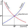
Demand curve is a graphical presentation of the "law of demand".[8] The curve shows how the price of a commodity or service changes as the quantity demanded increases. Every point on the curve is an amount of consumer demand and the corresponding market price. The graph shows the law of demand, which states that people will buy less of something if the price goes up and vice versa. According to Kotler, eight demand states are possible:
Negative demand — Consumers dislike the product and may even pay to avoid it.
Nonexistent demand — Consumers may be unaware of or uninterested in the product.
Latent demand — Consumers may share a strong need that cannot be satisfied by an existing product.
Declining demand — Consumers begin to buy the product less frequently or not at all.
Irregular demand — Consumer purchases vary on a seasonal, monthly, weekly, daily, or even hourly basis.
Full demand — Consumers are adequately buying all products put into the marketplace.
Overfull demand — More consumers would like to buy the product than can be satisfied.
Unwholesome demand — Consumers may be attracted to products that have undesirable social consequences.[9]
The price elasticity of demand is a measure of the sensitivity of the quantity variable, Q, to changes in the price variable, P. It shows the percent by which the quantity demanded will change as a result of a given percentage change in the price. Thus, a demand elasticity of -2 says that the quantity demanded will fall 2% if the price rises 1%. For infinitesimal changes, the elasticity is (∂Q/∂P)×(P/Q).
Elasticity along linear demand curve
The slope of a linear demand curve is constant. The elasticity of demand changes continuously as one moves down the demand curve because the ratio of price to quantity continuously falls. At the point the demand curve intersects the y-axis, demand becomes infinitely elastic, because the variable Q appearing in the denominator of the elasticity formula is zero. At the point the demand curve intersects the x-axis, the elasticity is zero, because the variable P appearing in the numerator of the elasticity formula is zero.[10] At one point on a linear demand curve, demand is unitary elastic: an elasticity of minus one. For higher prices, the elasticity is greater than -1 in magnitude: demand is said to be elastic because percentage quantity changes are bigger than price changes. For prices below the point of unit elasticity, the elasticity is less than -1 (-1<Ed<0) and demand is said to be inelastic.
Constant price elasticity demand
Constant elasticity of demand occurs when where a and c are parameters, and the constant price elasticity is
Perfectly inelastic demand
Perfectly inelastic demand is represented by a vertical demand curve. Under perfect price inelasticity of demand, the price has no effect on the quantity demanded. The demand for the good remains the same regardless of how low or high the price. Goods with (nearly) perfectly inelastic demand are typically goods with no substitutes. For instance, insulin is nearly perfectly inelastic. Diabetics need insulin to survive so a change in price would not effect the quantity demanded. Insulin is not perfectly inelastic, however, as a prohibitively high price would cause some individuals to be incapable of purchasing insulin entirely. On the other hand, if insulin was sold at a very low price, it is possible that some individuals would purchase more insulin if they were not able to afford it before. Because of the effects of extreme pricing, no good can be considered truly perfectly inelastic.
Market structure and the demand curve
In perfectly competitive markets the demand curve, the average revenue curve, and the marginal revenue curve all coincide and are horizontal at the market-given price.[11] The demand curve is perfectly elastic and coincides with the average and marginal revenue curves. Economic actors are price-takers. Perfectly competitive firms have zero market power; that is, they have no ability to affect the terms and conditions of exchange. A perfectly competitive firm's decisions are limited to whether to produce and if so, how much. In less than perfectly competitive markets the demand curve is negatively sloped and there is a separate marginal revenue curve. A firm in a less than perfectly competitive market is a price-setter. The firm can decide how much to produce or what price to charge. In deciding one variable the firm is necessarily determining the other variable
In its standard form a linear demand equation is Q = a - bP. That is, quantity demanded is a function of price. The inverse demand equation, or price equation, treats price as a function f of quantity demanded: P = f(Q). To compute the inverse demand equation, simply solve for P from the demand equation.[12] For example, if the demand equation is Q = 240 - 2P then the inverse demand equation would be P = 120 - .5Q, the right side of which is the inverse demand function.[13]
The inverse demand function is useful in deriving the total and marginal revenue functions. Total revenue equals price, P, times quantity, Q, or TR = P×Q. Multiply the inverse demand function by Q to derive the total revenue function: TR = (120 - .5Q) × Q = 120Q - 0.5Q². The marginal revenue function is the first derivative of the total revenue function; here MR = 120 - Q. Note that the MR function has the same y-intercept as the inverse demand function in this linear example; the x-intercept of the MR function is one-half the value of that of the demand function, and the slope of the MR function is twice that of the inverse demand function. This relationship holds true for all linear demand equations. The importance of being able to quickly calculate MR is that the profit-maximizing condition for firms regardless of market structure is to produce where marginal revenue equals marginal cost (MC). To derive MC the first derivative of the total cost function is taken. For example, assume cost, C, equals 420 + 60Q + Q2. Then MC = 60 + 2Q. Equating MR to MC and solving for Q gives Q = 20. So 20 is the profit maximizing quantity: to find the profit-maximizing price simply plug the value of Q into the inverse demand equation and solve for P.
Residual demand curve
The demand curve facing a particular firm is called the residual demand curve. The residual demand curve is the market demand that is not met by other firms in the industry at a given price. The residual demand curve is the market demand curve D(p), minus the supply of other organizations, So(p): Dr(p) = D(p) - So(p)[14]
Demand function and total revenue
If the demand curve is linear, then it has the form: Qd = a - b*P, where p is the price of the good and q is the quantity demanded. The intercept of the curve and the vertical axis is represented by a, meaning the price when no quantity demanded. and b is the slope of the demand function. If the demand function has the form like that, then the Total Revenue should equal quantity demanded times the price of the good, which can be represented by: TR= q*p = q(a-bq).
Is the demand curve for PC firm really flat?
Practically every introductory microeconomics text describes the demand curve facing a perfectly competitive firm as being flat or horizontal. A horizontal demand curve is perfectly elastic. If there are n identical firms in the market then the elasticity of demand PED facing any one firm is
PEDmi = nPEDm - (n - 1) PES
where PEDm is the market elasticity of demand, PES is the elasticity of supply of each of the other firms, and (n -1) is the number of other firms. This formula suggests two things. The demand curve is not perfectly elastic and if there are a large number of firms in the industry the elasticity of demand for any individual firm will be extremely high and the demand curve facing the firm will be nearly flat.[14]
For example, assume that there are 80 firms in the industry and that the demand elasticity for industry is -1.0 and the price elasticity of supply is 3. Then
PEDmi = (80 x (-1)) - (79 x 3) = -80 - 237 = -317
That is the firm PED is 317 times as elastic as the market PED. If a firm raised its price "by one tenth of one percent demand would drop by nearly one third."[14] if the firm raised its price by three tenths of one percent the quantity demanded would drop by nearly 100%. Three tenths of one percent marks the effective range of pricing power the firm has because any attempt to raise prices by a higher percentage will effectively reduce quantity demanded to zero.
Demand management has a defined set of processes, capabilities and recommended behaviors for companies that produce goods and services. Consumer electronics and goods companies often lead in the application of demand management practices to their demand chains; demand management outcomes are a reflection of policies and programs to influence demand as well as competition and options available to users and consumers. Effective demand management follows the concept of a "closed loop" where feedback from the results of the demand plans is fed back into the planning process to improve the predictability of outcomes. Many practices reflect elements of systems dynamics. Volatility is being recognized as significant an issue as the focus on variance of demand to plans and forecasts.
Different types of goods demand
Negative demand: If the market response to a product is negative, it shows that people are not aware of the features of the service and the benefits offered. Under such circumstances, the marketing unit of a service firm has to understand the psyche of the potential buyers and find out the prime reason for the rejection of the service. For example: if passengers refuse a bus conductor's call to board the bus. The service firm has to come up with an appropriate strategy to remove the misunderstandings of the potential buyers. A strategy needs to be designed to transform the negative demand into a positive demand.
No demand: If people are unaware, have insufficient information about a service or due to the consumer's indifference this type of a demand situation could occur. The marketing unit of the firm should focus on promotional campaigns and communicating reasons for potential customers to use the firm's services. Service differentiation is one of the popular strategies used to compete in a no demand situation in the market.
Latent demand: At any given time it is impossible to have a set of services that offer total satisfaction to all the needs and wants of society. In the market there exists a gap between desirable and the available. There is always a search on for better and newer offers to fill the gap between desirability and availability. Latent demand is a phenomenon of any economy at any given time, it should be looked upon as a business opportunity by service firms and they should orient themselves to identify and exploit such opportunities at the right time. For example, a passenger traveling in an ordinary bus dreams of traveling in a luxury bus. Therefore, latent demand is nothing but the gap between desirability and availability.
Seasonal demand: Some services do not have a year-round demand, and might be required only at a certain period of time. Seasons all over the world are diverse. Seasonal demands create many problems for service organizations, such as idling the capacity, fixed cost and excess expenditure on marketing and promotions. Strategies used by firms to overcome this may include nurturing the service consumption habit of customers so as to make the demand unseasonal, or recognizing markets elsewhere in the world during the off-season period. Hence, this presents an opportunity to target different markets with the appropriate season in different parts of the world. For example, the need for Christmas cards comes around once a year.
Demand patterns need to be studied in different segments of the market. Service organizations need to constantly study changing demands related to their service offerings over various time periods. They have to develop a system to chart these demand fluctuations, which helps them in predicting the demand cycles. Demands do fluctuate randomly; therefore, they should be followed on a daily, weekly or monthly basis.
Criticism
E. F. Schumacher challenges the prevailing economic assumption that fulfilling demand is the purpose of economic activity, offering a framework of what he calls "Buddhist economics" in which wise demands, fulfilling genuine human needs, are distinguished from unwise demands, arising from the five intellectual impairments recognized by Buddhism:[15]
The cultivation and expansion of needs is the antithesis of wisdom. It is also the antithesis of freedom and peace. Every increase of needs tends to increase one's dependence on outside forces over which one cannot have control, and therefore increases existential fear. Only by a reduction of needs can one promote a genuine reduction in those tensions which are the ultimate causes of strife and war.[16]
Demand reduction refers to efforts aimed at reducing the public desire for illegal and illicit drugs. The drug policy is in contrast to the reduction of drug supply, but the two policies are often implemented together.
Energy demand management, also known as demand-side management (DSM) or demand-side response (DSR), is the modification of consumer demand for energy through various methods such as financial incentives and behavioral change through education.
↑ Kotler, Philip & Keller, Kevin L. (2015). Marketing Management, 15th Edition. Harlow, Pearson ISBN1-292-09262-9
↑ Colander, David C. Microeconomics 7th ed. pp. 132–133. McGraw-Hill 2008.
↑ The perfectly competitive firm's demand curve is not in fact flat. However, if there are numerous firms in the industry the demand curve of an individual firm is likely to be extremely elastic, for a discussion of residual demand curves see Perloff (2008) at pp. 245–246.
↑ The form of the inverse linear demand equation is P = a/b - 1/bQ.
↑ Samuelson, W & Marks, S. Managerial Economics 4th ed. p. 37. Wiley 2003.
This page is based on this Wikipedia article Text is available under the CC BY-SA 4.0 license; additional terms may apply. Images, videos and audio are available under their respective licenses.