A monopoly, as described by Irving Fisher, is a market with the "absence of competition", creating a situation where a specific person or enterprise is the only supplier of a particular thing. This contrasts with a monopsony which relates to a single entity's control of a market to purchase a good or service, and with oligopoly and duopoly which consists of a few sellers dominating a market. Monopolies are thus characterised by a lack of economic competition to produce the good or service, a lack of viable substitute goods, and the possibility of a high monopoly price well above the seller's marginal cost that leads to a high monopoly profit. The verb monopolise or monopolize refers to the process by which a company gains the ability to raise prices or exclude competitors. In economics, a monopoly is a single seller. In law, a monopoly is a business entity that has significant market power, that is, the power to charge overly high prices, which is associated with unfair price raises. Although monopolies may be big businesses, size is not a characteristic of a monopoly. A small business may still have the power to raise prices in a small industry.
An oligopoly is a market in which pricing control lies in the hands of a few sellers.

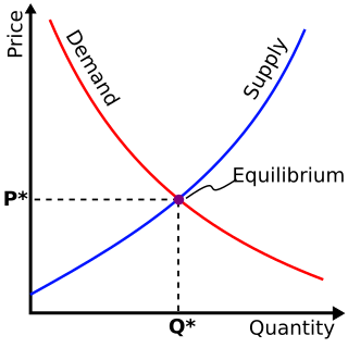
In microeconomics, supply and demand is an economic model of price determination in a market. It postulates that, holding all else equal, the unit price for a particular good or other traded item in a perfectly competitive market, will vary until it settles at the market-clearing price, where the quantity demanded equals the quantity supplied such that an economic equilibrium is achieved for price and quantity transacted. The concept of supply and demand forms the theoretical basis of modern economics.

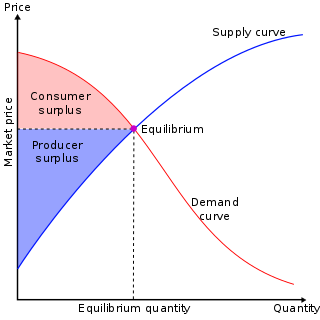
In mainstream economics, economic surplus, also known as total welfare or total social welfare or Marshallian surplus, is either of two related quantities:

In economics, profit maximization is the short run or long run process by which a firm may determine the price, input and output levels that will lead to the highest possible total profit. In neoclassical economics, which is currently the mainstream approach to microeconomics, the firm is assumed to be a "rational agent" which wants to maximize its total profit, which is the difference between its total revenue and its total cost.

In economics, elasticity measures the responsiveness of one economic variable to a change in another. For example, if the price elasticity of the demand of a good is -2, then a 10% increase in price will cause the quantity demanded to fall by 20%. Elasticity in economics provides an understanding of changes in the behavior of the buyers and sellers with price changes. There are two types of elasticity for demand and supply, one is inelastic demand and supply and the other one is elastic demand and supply.
A good's price elasticity of demand is a measure of how sensitive the quantity demanded is to its price. When the price rises, quantity demanded falls for almost any good, but it falls more for some than for others. The price elasticity gives the percentage change in quantity demanded when there is a one percent increase in price, holding everything else constant. If the elasticity is −2, that means a one percent price rise leads to a two percent decline in quantity demanded. Other elasticities measure how the quantity demanded changes with other variables.
In economics, the marginal cost is the change in the total cost that arises when the quantity produced is increased, i.e. the cost of producing additional quantity. In some contexts, it refers to an increment of one unit of output, and in others it refers to the rate of change of total cost as output is increased by an infinitesimal amount. As Figure 1 shows, the marginal cost is measured in dollars per unit, whereas total cost is in dollars, and the marginal cost is the slope of the total cost, the rate at which it increases with output. Marginal cost is different from average cost, which is the total cost divided by the number of units produced.
Managerial economics is a branch of economics involving the application of economic methods in the organizational decision-making process. Economics is the study of the production, distribution, and consumption of goods and services. Managerial economics involves the use of economic theories and principles to make decisions regarding the allocation of scarce resources. It guides managers in making decisions relating to the company's customers, competitors, suppliers, and internal operations.

In economics, comparative statics is the comparison of two different economic outcomes, before and after a change in some underlying exogenous parameter.

A demand curve is a graph depicting the inverse demand function, a relationship between the price of a certain commodity and the quantity of that commodity that is demanded at that price. Demand curves can be used either for the price-quantity relationship for an individual consumer, or for all consumers in a particular market.

Marginal revenue is a central concept in microeconomics that describes the additional total revenue generated by increasing product sales by 1 unit. Marginal revenue is the increase in revenue from the sale of one additional unit of product, i.e., the revenue from the sale of the last unit of product. It can be positive or negative. Marginal revenue is an important concept in vendor analysis. To derive the value of marginal revenue, it is required to examine the difference between the aggregate benefits a firm received from the quantity of a good and service produced last period and the current period with one extra unit increase in the rate of production. Marginal revenue is a fundamental tool for economic decision making within a firm's setting, together with marginal cost to be considered.
Cournot competition is an economic model used to describe an industry structure in which companies compete on the amount of output they will produce, which they decide on independently of each other and at the same time. It is named after Antoine Augustin Cournot (1801–1877) who was inspired by observing competition in a spring water duopoly. It has the following features:
In economics, a cost curve is a graph of the costs of production as a function of total quantity produced. In a free market economy, productively efficient firms optimize their production process by minimizing cost consistent with each possible level of production, and the result is a cost curve. Profit-maximizing firms use cost curves to decide output quantities. There are various types of cost curves, all related to each other, including total and average cost curves; marginal cost curves, which are equal to the differential of the total cost curves; and variable cost curves. Some are applicable to the short run, others to the long run.
In economics, the long-run is a theoretical concept in which all markets are in equilibrium, and all prices and quantities have fully adjusted and are in equilibrium. The long-run contrasts with the short-run, in which there are some constraints and markets are not fully in equilibrium. More specifically, in microeconomics there are no fixed factors of production in the long-run, and there is enough time for adjustment so that there are no constraints preventing changing the output level by changing the capital stock or by entering or leaving an industry. This contrasts with the short-run, where some factors are variable and others are fixed, constraining entry or exit from an industry. In macroeconomics, the long-run is the period when the general price level, contractual wage rates, and expectations adjust fully to the state of the economy, in contrast to the short-run when these variables may not fully adjust.

In economics, demand is the quantity of a good that consumers are willing and able to purchase at various prices during a given time. In economics "demand" for a commodity is not the same thing as "desire" for it. It refers to both the desire to purchase and the ability to pay for a commodity.

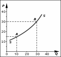
In economics, supply is the amount of a resource that firms, producers, labourers, providers of financial assets, or other economic agents are willing and able to provide to the marketplace or to an individual. Supply can be in produced goods, labour time, raw materials, or any other scarce or valuable object. Supply is often plotted graphically as a supply curve, with the price per unit on the vertical axis and quantity supplied as a function of price on the horizontal axis. This reversal of the usual position of the dependent variable and the independent variable is an unfortunate but standard convention.
A firm will choose to implement a shutdown of production when the revenue received from the sale of the goods or services produced cannot even cover the variable costs of production. In that situation, the firm will experience a higher loss when it produces, compared to not producing at all.
In economics, the marginal product of labor (MPL) is the change in output that results from employing an added unit of labor. It is a feature of the production function and depends on the amounts of physical capital and labor already in use.

In microeconomics, a monopoly price is set by a monopoly. A monopoly occurs when a firm lacks any viable competition and is the sole producer of the industry's product. Because a monopoly faces no competition, it has absolute market power and can set a price above the firm's marginal cost.


