Econometrics

For broader coverage of this topic, see Mathematical economics.

Econometrics is an application of statistical methods to economic data in order to give empirical content to economic relationships. ^[1] More precisely, it is "the quantitative analysis of actual economic phenomena based on the concurrent development of theory and observation, related by appropriate methods of inference." ^[2] An introductory economics textbook describes econometrics as allowing economists "to sift through mountains of data to extract simple relationships." ^[3] Jan Tinbergen is one of the two founding fathers of econometrics. ^{[4] [5] [6]} The other, Ragnar Frisch, also coined the term in the sense in which it is used today. ^[7]

A basic tool for econometrics is the multiple linear regression model. ^[8] Econometric theory uses statistical theory and mathematical statistics to evaluate and develop econometric methods. ^{[9] [10]} Econometricians try to find estimators that have desirable statistical properties including unbiasedness, efficiency, and consistency. Applied econometrics uses theoretical econometrics and real-world data for assessing economic theories, developing econometric models, analysing economic history, and forecasting.

Basic models: linear regression

A basic tool for econometrics is the multiple linear regression model. ^[8] In modern econometrics, other statistical tools are frequently used, but linear regression is still the most frequently used starting point for an analysis. ^[8] Estimating a linear regression on two variables can be visualized as fitting a line through data points representing paired values of the independent and dependent variables.

Okun's law representing the relationship between GDP growth and the unemployment rate. The fitted line is found using regression analysis.

For example, consider Okun's law, which relates GDP growth to the unemployment rate. This relationship is represented in a linear regression where the change in unemployment rate (${\displaystyle \Delta \ {\text{Unemployment}}}$) is a function of an intercept (${\displaystyle \beta _{0}}$), a given value of GDP growth multiplied by a slope coefficient ${\displaystyle \beta _{1}}$ and an error term, ${\displaystyle \varepsilon }$:

${\displaystyle \Delta \ {\text{Unemployment}}=\beta _{0}+\beta _{1}{\text{Growth}}+\varepsilon .}$

The unknown parameters ${\displaystyle \beta _{0}}$ and ${\displaystyle \beta _{1}}$ can be estimated. Here ${\displaystyle \beta _{0}}$ is estimated to be 0.83 and ${\displaystyle \beta _{1}}$ is estimated to be -1.77. This means that if GDP growth increased by one percentage point, the unemployment rate would be predicted to drop by 1.77 * 1 points, other things held constant. The model could then be tested for statistical significance as to whether an increase in GDP growth is associated with a decrease in the unemployment, as hypothesized. If the estimate of ${\displaystyle \beta _{1}}$ were not significantly different from 0, the test would fail to find evidence that changes in the growth rate and unemployment rate were related. The variance in a prediction of the dependent variable (unemployment) as a function of the independent variable (GDP growth) is given in polynomial least squares.

Theory

See also: Estimation theory

Econometric theory uses statistical theory and mathematical statistics to evaluate and develop econometric methods. ^{[9] [10]} Econometricians try to find estimators that have desirable statistical properties including unbiasedness, efficiency, and consistency. An estimator is unbiased if its expected value is the true value of the parameter; it is consistent if it converges to the true value as the sample size gets larger, and it is efficient if the estimator has lower standard error than other unbiased estimators for a given sample size. Ordinary least squares (OLS) is often used for estimation since it provides the BLUE or "best linear unbiased estimator" (where "best" means most efficient, unbiased estimator) given the Gauss-Markov assumptions. When these assumptions are violated or other statistical properties are desired, other estimation techniques such as maximum likelihood estimation, generalized method of moments, or generalized least squares are used. Estimators that incorporate prior beliefs are advocated by those who favour Bayesian statistics over traditional, classical or "frequentist" approaches.

Methods

Main article: Methodology of econometrics

Applied econometrics uses theoretical econometrics and real-world data for assessing economic theories, developing econometric models, analysing economic history, and forecasting. ^[11]

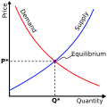
Econometrics uses standard statistical models to study economic questions, but most often these are based on observational data, rather than data from controlled experiments. ^[12] In this, the design of observational studies in econometrics is similar to the design of studies in other observational disciplines, such as astronomy, epidemiology, sociology and political science. Analysis of data from an observational study is guided by the study protocol, although exploratory data analysis may be useful for generating new hypotheses. ^[13] Economics often analyses systems of equations and inequalities, such as supply and demand hypothesized to be in equilibrium. Consequently, the field of econometrics has developed methods for identification and estimation of simultaneous equations models. These methods are analogous to methods used in other areas of science, such as the field of system identification in systems analysis and control theory. Such methods may allow researchers to estimate models and investigate their empirical consequences, without directly manipulating the system.

In the absence of evidence from controlled experiments, econometricians often seek illuminating natural experiments or apply quasi-experimental methods to draw credible causal inference. ^[14] The methods include regression discontinuity design, instrumental variables, and difference-in-differences.

Example

A simple example of a relationship in econometrics from the field of labour economics is:

${\displaystyle \ln({\text{wage}})=\beta _{0}+\beta _{1}({\text{years of education}})+\varepsilon .}$

This example assumes that the natural logarithm of a person's wage is a linear function of the number of years of education that person has acquired. The parameter ${\displaystyle \beta _{1}}$ measures the increase in the natural log of the wage attributable to one more year of education. The term ${\displaystyle \varepsilon }$ is a random variable representing all other factors that may have direct influence on wage. The econometric goal is to estimate the parameters, ${\displaystyle \beta _{0}{\mbox{ and }}\beta _{1}}$ under specific assumptions about the random variable ${\displaystyle \varepsilon }$. For example, if ${\displaystyle \varepsilon }$ is uncorrelated with years of education, then the equation can be estimated with ordinary least squares.

If the researcher could randomly assign people to different levels of education, the data set thus generated would allow estimation of the effect of changes in years of education on wages. In reality, those experiments cannot be conducted. Instead, the econometrician observes the years of education of and the wages paid to people who differ along many dimensions. Given this kind of data, the estimated coefficient on years of education in the equation above reflects both the effect of education on wages and the effect of other variables on wages, if those other variables were correlated with education. For example, people born in certain places may have higher wages and higher levels of education. Unless the econometrician controls for place of birth in the above equation, the effect of birthplace on wages may be falsely attributed to the effect of education on wages.

The most obvious way to control for birthplace is to include a measure of the effect of birthplace in the equation above. Exclusion of birthplace, together with the assumption that ${\displaystyle \epsilon }$ is uncorrelated with education produces a misspecified model. Another technique is to include in the equation additional set of measured covariates which are not instrumental variables, yet render ${\displaystyle \beta _{1}}$ identifiable. ^[15] An overview of econometric methods used to study this problem were provided by Card (1999). ^[16]

Journals

The main journals that publish work in econometrics are:

• Econometrica , which is published by Econometric Society. ^[17]
• The Review of Economics and Statistics , which is over 100 years old. ^[18]
• The Econometrics Journal , which was established by the Royal Economic Society. ^[19]
• The Journal of Econometrics , which also publishes the supplement Annals of Econometrics. ^[20]
• Econometric Theory , which is a theoretical journal. ^[21]
• The Journal of Applied Econometrics , which applies econometrics to a wide various problems. ^[22]
• Econometric Reviews , which includes reviews on econometric books and software as well. ^[23]
• The Journal of Business & Economic Statistics, which is published by the American Statistical Association. ^[24]

Limitations and criticisms

See also: Criticisms of econometrics

Like other forms of statistical analysis, badly specified econometric models may show a spurious relationship where two variables are correlated but causally unrelated. In a study of the use of econometrics in major economics journals, McCloskey concluded that some economists report p-values (following the Fisherian tradition of tests of significance of point null-hypotheses) and neglect concerns of type II errors; some economists fail to report estimates of the size of effects (apart from statistical significance) and to discuss their economic importance. She also argues that some economists also fail to use economic reasoning for model selection, especially for deciding which variables to include in a regression. ^{[25] [26]}

In some cases, economic variables cannot be experimentally manipulated as treatments randomly assigned to subjects. ^[27] In such cases, economists rely on observational studies, often using data sets with many strongly associated covariates, resulting in enormous numbers of models with similar explanatory ability but different covariates and regression estimates. Regarding the plurality of models compatible with observational data-sets, Edward Leamer urged that "professionals ... properly withhold belief until an inference can be shown to be adequately insensitive to the choice of assumptions". ^[27]

See also

• Choice modelling
• Cowles Foundation
• Econometric software
• Financial econometrics
• Financial modeling
• Important publications in econometrics
• Single-equation methods (econometrics)

Further reading

• Econometric Theory book on Wikibooks
• Giovannini, Enrico Understanding Economic Statistics, OECD Publishing, 2008, ISBN   978-92-64-03312-2

References

1. M. Hashem Pesaran (1987). "Econometrics", The New Palgrave: A Dictionary of Economics , v. 2, p. 8 [pp. 8–22]. Reprinted in J. Eatwell et al., eds. (1990). Econometrics: The New Palgrave, p. 1 Archived 15 March 2023 at the Wayback Machine [pp. 1–34]. Abstract Archived 18 May 2012 at the Wayback Machine (2008 revision by J. Geweke, J. Horowitz, and H. P. Pesaran).
2. P. A. Samuelson, T. C. Koopmans, and J. R. N. Stone (1954). "Report of the Evaluative Committee for Econometrica", Econometrica 22(2), p. 142. [p p. 141-146], as described and cited in Pesaran (1987) above.
3. Paul A. Samuelson and William D. Nordhaus, 2004. Economics . 18th ed., McGraw-Hill, p. 5.
4. "1969 - Jan Tinbergen: Nobelprijs economie - Elsevierweekblad.nl". elsevierweekblad.nl. 12 October 2015. Archived from the original on 1 May 2018. Retrieved 1 May 2018.
5. Magnus, Jan & Mary S. Morgan (1987) The ET Interview: Professor J. Tinbergen in: 'Econometric Theory 3, 1987, 117–142.
6. Willlekens, Frans (2008) International Migration in Europe: Data, Models and Estimates. New Jersey. John Wiley & Sons: 117.
7. • H. P. Pesaran (1990), "Econometrics", Econometrics: The New Palgrave, p. 2 Archived 15 March 2023 at the Wayback Machine , citing Ragnar Frisch (1936), "A Note on the Term 'Econometrics'", Econometrica, 4(1), p. 95.
      • Aris Spanos (2008), "statistics and economics", The New Palgrave Dictionary of Economics , 2nd Edition. Abstract. Archived 18 May 2012 at the Wayback Machine
8. Greene, William (2012). "Chapter 1: Econometrics". Econometric Analysis (7th ed.). Pearson Education. pp. 47–48. ISBN   9780273753568. Ultimately, all of these will require a common set of tools, including, for example, the multiple regression model, the use of moment conditions for estimation, instrumental variables (IV) and maximum likelihood estimation. With that in mind, the organization of this book is as follows: The first half of the text develops fundamental results that are common to all the applications. The concept of multiple regression and the linear regression model in particular constitutes the underlying platform of most modeling, even if the linear model itself is not ultimately used as the empirical specification.
9. Greene, William (2012). Econometric Analysis (7th ed.). Pearson Education. pp. 34, 41–42. ISBN   9780273753568.
10. Wooldridge, Jeffrey (2012). "Chapter 1: The Nature of Econometrics and Economic Data". Introductory Econometrics: A Modern Approach (5th ed.). South-Western Cengage Learning. p. 2. ISBN   9781111531041.
11. Clive Granger (2008). "forecasting", The New Palgrave Dictionary of Economics, 2nd Edition. Abstract. Archived 18 May 2012 at the Wayback Machine
12. Wooldridge, Jeffrey (2013). Introductory Econometrics, A modern approach. South-Western, Cengage learning. ISBN   978-1-111-53104-1.
13. Herman O. Wold (1969). "Econometrics as Pioneering in Nonexperimental Model Building", Econometrica, 37(3), pp. 369 Archived 24 August 2017 at the Wayback Machine -381.
14. Angrist, Joshua D.; Pischke, Jörn-Steffen (May 2010). "The Credibility Revolution in Empirical Economics: How Better Research Design is Taking the Con out of Econometrics". Journal of Economic Perspectives. 24 (2): 3–30. doi: 10.1257/jep.24.2.3 . hdl: 1721.1/54195 . ISSN   0895-3309.
15. Pearl, Judea (2000). Causality: Model, Reasoning, and Inference . Cambridge University Press. ISBN   978-0521773621.
16. Card, David (1999). "The Causal Effect of Education on Earning". In Ashenfelter, O.; Card, D. (eds.). Handbook of Labor Economics. Amsterdam: Elsevier. pp. 1801–1863. ISBN   978-0444822895.
17. "Home". www.econometricsociety.org. Retrieved 14 February 2024.
18. "The Review of Economics and Statistics". direct.mit.edu. Retrieved 14 February 2024.
19. "The Econometrics Journal". Wiley.com. Archived from the original on 6 October 2011. Retrieved 8 October 2013.
20. "Journal of Econometrics". www.scimagojr.com. Retrieved 14 February 2024.
21. "Home" . Retrieved 14 March 2024.
22. "Journal of Applied Econometrics". Journal of Applied Econometrics.
23. Econometric Reviews Print ISSN: 0747-4938 Online ISSN: 1532-4168 https://www.tandfonline.com/action/journalInformation?journalCode=lecr20
24. "Journals". Default. Retrieved 14 February 2024.
25. McCloskey (May 1985). "The Loss Function has been mislaid: the Rhetoric of Significance Tests". American Economic Review. 75 (2).
26. Stephen T. Ziliak and Deirdre N. McCloskey (2004). "Size Matters: The Standard Error of Regressions in the American Economic Review", Journal of Socio-Economics, 33(5), pp. 527-46 Archived 25 June 2010 at the Wayback Machine (press +).
27. Leamer, Edward (March 1983). "Let's Take the Con out of Econometrics". American Economic Review. 73 (1): 31–43. JSTOR   1803924.

External links

• Journal of Financial Econometrics
• Econometric Society
• The Econometrics Journal
• Econometric Links
• Teaching Econometrics (Index by the Economics Network (UK))
• Applied Econometric Association
• The Society for Financial Econometrics
• The interview with Clive Granger – Nobel winner in 2003, about econometrics