Econometrics is an application of statistical methods to economic data in order to give empirical content to economic relationships. More precisely, it is "the quantitative analysis of actual economic phenomena based on the concurrent development of theory and observation, related by appropriate methods of inference." An introductory economics textbook describes econometrics as allowing economists "to sift through mountains of data to extract simple relationships." Jan Tinbergen is one of the two founding fathers of econometrics. The other, Ragnar Frisch, also coined the term in the sense in which it is used today.
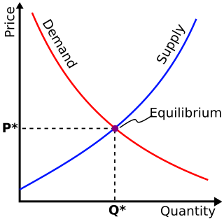
In microeconomics, supply and demand is an economic model of price determination in a market. It postulates that, holding all else equal, the unit price for a particular good or other traded item in a perfectly competitive market, will vary until it settles at the market-clearing price, where the quantity demanded equals the quantity supplied such that an economic equilibrium is achieved for price and quantity transacted. The concept of supply and demand forms the theoretical basis of modern economics.
Simultaneous equations models are a type of statistical model in which the dependent variables are functions of other dependent variables, rather than just independent variables. This means some of the explanatory variables are jointly determined with the dependent variable, which in economics usually is the consequence of some underlying equilibrium mechanism. Take the typical supply and demand model: whilst typically one would determine the quantity supplied and demanded to be a function of the price set by the market, it is also possible for the reverse to be true, where producers observe the quantity that consumers demand and then set the price.

In economics, comparative statics is the comparison of two different economic outcomes, before and after a change in some underlying exogenous parameter.
A demand curve is a graph depicting the inverse demand function, a relationship between the price of a certain commodity and the quantity of that commodity that is demanded at that price. Demand curves can be used either for the price-quantity relationship for an individual consumer, or for all consumers in a particular market.
Econometric models are statistical models used in econometrics. An econometric model specifies the statistical relationship that is believed to hold between the various economic quantities pertaining to a particular economic phenomenon. An econometric model can be derived from a deterministic economic model by allowing for uncertainty, or from an economic model which itself is stochastic. However, it is also possible to use econometric models that are not tied to any specific economic theory.
In statistics, and particularly in econometrics, the reduced form of a system of equations is the result of solving the system for the endogenous variables. This gives the latter as functions of the exogenous variables, if any. In econometrics, the equations of a structural form model are estimated in their theoretically given form, while an alternative approach to estimation is to first solve the theoretical equations for the endogenous variables to obtain reduced form equations, and then to estimate the reduced form equations.
In statistics, econometrics, epidemiology and related disciplines, the method of instrumental variables (IV) is used to estimate causal relationships when controlled experiments are not feasible or when a treatment is not successfully delivered to every unit in a randomized experiment. Intuitively, IVs are used when an explanatory variable of interest is correlated with the error term (endogenous), in which case ordinary least squares and ANOVA give biased results. A valid instrument induces changes in the explanatory variable but has no independent effect on the dependent variable and is not correlated with the error term, allowing a researcher to uncover the causal effect of the explanatory variable on the dependent variable.
In econometrics, endogeneity broadly refers to situations in which an explanatory variable is correlated with the error term. The distinction between endogenous and exogenous variables originated in simultaneous equations models, where one separates variables whose values are determined by the model from variables which are predetermined. Ignoring simultaneity in the estimation leads to biased estimates as it violates the exogeneity assumption of the Gauss–Markov theorem. The problem of endogeneity is often ignored by researchers conducting non-experimental research and doing so precludes making policy recommendations. Instrumental variable techniques are commonly used to mitigate this problem.
In econometrics and statistics, the generalized method of moments (GMM) is a generic method for estimating parameters in statistical models. Usually it is applied in the context of semiparametric models, where the parameter of interest is finite-dimensional, whereas the full shape of the data's distribution function may not be known, and therefore maximum likelihood estimation is not applicable.
In economics, demand is the quantity of a good that consumers are willing and able to purchase at various prices during a given time. In economics "demand" for a commodity is not the same thing as "desire" for it. It refers to both the desire to purchase and the ability to pay for a commodity.
The Heckman correction is a statistical technique to correct bias from non-randomly selected samples or otherwise incidentally truncated dependent variables, a pervasive issue in quantitative social sciences when using observational data. Conceptually, this is achieved by explicitly modelling the individual sampling probability of each observation together with the conditional expectation of the dependent variable. The resulting likelihood function is mathematically similar to the tobit model for censored dependent variables, a connection first drawn by James Heckman in 1974. Heckman also developed a two-step control function approach to estimate this model, which avoids the computational burden of having to estimate both equations jointly, albeit at the cost of inefficiency. Heckman received the Nobel Memorial Prize in Economic Sciences in 2000 for his work in this field.
Jacques H. Drèze was a Belgian economist noted for his contributions to economic theory, econometrics, and economic policy as well as for his leadership in the economics profession. Drèze was the first President of the European Economic Association in 1986 and was the President of the Econometric Society in 1970.

In statistics, errors-in-variables models or measurement error models are regression models that account for measurement errors in the independent variables. In contrast, standard regression models assume that those regressors have been measured exactly, or observed without error; as such, those models account only for errors in the dependent variables, or responses.
The methodology of econometrics is the study of the range of differing approaches to undertaking econometric analysis.
Teunis (Teun) Kloek is a Dutch economist and Emeritus Professor of Econometrics at the Erasmus Universiteit Rotterdam. His research interests centered on econometric methods and their applications, especially nonparametric and robust methods in econometrics.
Philip Green Wright was an American economist who in 1928 first proposed the use of instrumental variables estimation as the earliest known solution to the identification problem in econometrics. In a book review published in 1915 he wrote one of the first explanations of the identification problem. His primary topic of applied research was tariff policy, and he wrote several books on the topic. He also wrote poetry, was a mentor to the poet and author Carl Sandburg, and published some of Sandburg's earliest works. Wright was the father of geneticist Sewall Wright.
Control functions are statistical methods to correct for endogeneity problems by modelling the endogeneity in the error term. The approach thereby differs in important ways from other models that try to account for the same econometric problem. Instrumental variables, for example, attempt to model the endogenous variable X as an often invertible model with respect to a relevant and exogenous instrument Z. Panel analysis uses special data properties to difference out unobserved heterogeneity that is assumed to be fixed over time.
In statistics and econometrics, set identification extends the concept of identifiability in statistical models to environments where the model and the distribution of observable variables are not sufficient to determine a unique value for the model parameters, but instead constrain the parameters to lie in a strict subset of the parameter space. Statistical models that are set identified arise in a variety of settings in economics, including game theory and the Rubin causal model. Unlike approaches that deliver point-identification of the model parameters, methods from the literature on partial identification are used to obtain set estimates that are valid under weaker modelling assumptions.


