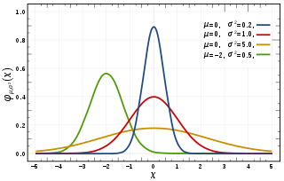
In statistics, a location parameter of a probability distribution is a scalar- or vector-valued parameter , which determines the "location" or shift of the distribution. In the literature of location parameter estimation, the probability distributions with such parameter are found to be formally defined in one of the following equivalent ways:

In probability theory and statistics, a normal distribution or Gaussian distribution is a type of continuous probability distribution for a real-valued random variable. The general form of its probability density function is The parameter is the mean or expectation of the distribution, while the parameter is the variance. The standard deviation of the distribution is (sigma). A random variable with a Gaussian distribution is said to be normally distributed, and is called a normal deviate.
A statistical model is a mathematical model that embodies a set of statistical assumptions concerning the generation of sample data. A statistical model represents, often in considerably idealized form, the data-generating process. When referring specifically to probabilities, the corresponding term is probabilistic model. All statistical hypothesis tests and all statistical estimators are derived via statistical models. More generally, statistical models are part of the foundation of statistical inference. A statistical model is usually specified as a mathematical relationship between one or more random variables and other non-random variables. As such, a statistical model is "a formal representation of a theory".
In statistics, the likelihood-ratio test is a hypothesis test that involves comparing the goodness of fit of two competing statistical models, typically one found by maximization over the entire parameter space and another found after imposing some constraint, based on the ratio of their likelihoods. If the more constrained model is supported by the observed data, the two likelihoods should not differ by more than sampling error. Thus the likelihood-ratio test tests whether this ratio is significantly different from one, or equivalently whether its natural logarithm is significantly different from zero.
In statistics, maximum likelihood estimation (MLE) is a method of estimating the parameters of an assumed probability distribution, given some observed data. This is achieved by maximizing a likelihood function so that, under the assumed statistical model, the observed data is most probable. The point in the parameter space that maximizes the likelihood function is called the maximum likelihood estimate. The logic of maximum likelihood is both intuitive and flexible, and as such the method has become a dominant means of statistical inference.
In mathematics, a Gaussian function, often simply referred to as a Gaussian, is a function of the base form and with parametric extension for arbitrary real constants a, b and non-zero c. It is named after the mathematician Carl Friedrich Gauss. The graph of a Gaussian is a characteristic symmetric "bell curve" shape. The parameter a is the height of the curve's peak, b is the position of the center of the peak, and c controls the width of the "bell".
In information geometry, the Fisher information metric is a particular Riemannian metric which can be defined on a smooth statistical manifold, i.e., a smooth manifold whose points are probability measures defined on a common probability space. It can be used to calculate the informational difference between measurements.
In mathematical statistics, the Fisher information is a way of measuring the amount of information that an observable random variable X carries about an unknown parameter θ of a distribution that models X. Formally, it is the variance of the score, or the expected value of the observed information.
In mathematical statistics, the Kullback–Leibler (KL) divergence, denoted , is a type of statistical distance: a measure of how one reference probability distribution P is different from a second probability distribution Q. Mathematically, it is defined as

In statistics, a consistent estimator or asymptotically consistent estimator is an estimator—a rule for computing estimates of a parameter θ0—having the property that as the number of data points used increases indefinitely, the resulting sequence of estimates converges in probability to θ0. This means that the distributions of the estimates become more and more concentrated near the true value of the parameter being estimated, so that the probability of the estimator being arbitrarily close to θ0 converges to one.
Estimation theory is a branch of statistics that deals with estimating the values of parameters based on measured empirical data that has a random component. The parameters describe an underlying physical setting in such a way that their value affects the distribution of the measured data. An estimator attempts to approximate the unknown parameters using the measurements. In estimation theory, two approaches are generally considered:
In Bayesian statistics, a maximum a posteriori probability (MAP) estimate is an estimate of an unknown quantity, that equals the mode of the posterior distribution. The MAP can be used to obtain a point estimate of an unobserved quantity on the basis of empirical data. It is closely related to the method of maximum likelihood (ML) estimation, but employs an augmented optimization objective which incorporates a prior distribution over the quantity one wants to estimate. MAP estimation can therefore be seen as a regularization of maximum likelihood estimation.
In statistics, the Bayesian information criterion (BIC) or Schwarz information criterion is a criterion for model selection among a finite set of models; models with lower BIC are generally preferred. It is based, in part, on the likelihood function and it is closely related to the Akaike information criterion (AIC).
In statistics, a parametric model or parametric family or finite-dimensional model is a particular class of statistical models. Specifically, a parametric model is a family of probability distributions that has a finite number of parameters.
Covariance matrix adaptation evolution strategy (CMA-ES) is a particular kind of strategy for numerical optimization. Evolution strategies (ES) are stochastic, derivative-free methods for numerical optimization of non-linear or non-convex continuous optimization problems. They belong to the class of evolutionary algorithms and evolutionary computation. An evolutionary algorithm is broadly based on the principle of biological evolution, namely the repeated interplay of variation and selection: in each generation (iteration) new individuals are generated by variation of the current parental individuals, usually in a stochastic way. Then, some individuals are selected to become the parents in the next generation based on their fitness or objective function value . Like this, individuals with better and better -values are generated over the generation sequence.
A ratio distribution is a probability distribution constructed as the distribution of the ratio of random variables having two other known distributions. Given two random variables X and Y, the distribution of the random variable Z that is formed as the ratio Z = X/Y is a ratio distribution.
In probability and statistics, the class of exponential dispersion models (EDM), also called exponential dispersion family (EDF), is a set of probability distributions that represents a generalisation of the natural exponential family. Exponential dispersion models play an important role in statistical theory, in particular in generalized linear models because they have a special structure which enables deductions to be made about appropriate statistical inference.
In statistics, the variance function is a smooth function that depicts the variance of a random quantity as a function of its mean. The variance function is a measure of heteroscedasticity and plays a large role in many settings of statistical modelling. It is a main ingredient in the generalized linear model framework and a tool used in non-parametric regression, semiparametric regression and functional data analysis. In parametric modeling, variance functions take on a parametric form and explicitly describe the relationship between the variance and the mean of a random quantity. In a non-parametric setting, the variance function is assumed to be a smooth function.

In machine learning, a variational autoencoder (VAE) is an artificial neural network architecture introduced by Diederik P. Kingma and Max Welling. It is part of the families of probabilistic graphical models and variational Bayesian methods.
The reparameterization trick is a technique used in statistical machine learning, particularly in variational inference, variational autoencoders, and stochastic optimization. It allows for the efficient computation of gradients through random variables, enabling the optimization of parametric probability models using stochastic gradient descent, and the variance reduction of estimators.


