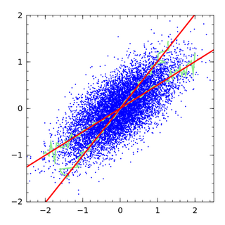
In statistics, the Gauss–Markov theorem states that the ordinary least squares (OLS) estimator has the lowest sampling variance within the class of linear unbiased estimators, if the errors in the linear regression model are uncorrelated, have equal variances and expectation value of zero. The errors do not need to be normal, nor do they need to be independent and identically distributed. The requirement that the estimator be unbiased cannot be dropped, since biased estimators exist with lower variance. See, for example, the James–Stein estimator, ridge regression, or simply any degenerate estimator.

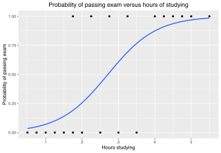
In statistics, the logistic model is a statistical model that models the log-odds of an event as a linear combination of one or more independent variables. In regression analysis, logistic regression estimates the parameters of a logistic model. In binary logistic regression there is a single binary dependent variable, coded by an indicator variable, where the two values are labeled "0" and "1", while the independent variables can each be a binary variable or a continuous variable. The corresponding probability of the value labeled "1" can vary between 0 and 1, hence the labeling; the function that converts log-odds to probability is the logistic function, hence the name. The unit of measurement for the log-odds scale is called a logit, from logistic unit, hence the alternative names. See § Background and § Definition for formal mathematics, and § Example for a worked example.

In statistical modeling, regression analysis is a set of statistical processes for estimating the relationships between a dependent variable and one or more error-free independent variables. The most common form of regression analysis is linear regression, in which one finds the line that most closely fits the data according to a specific mathematical criterion. For example, the method of ordinary least squares computes the unique line that minimizes the sum of squared differences between the true data and that line. For specific mathematical reasons, this allows the researcher to estimate the conditional expectation of the dependent variable when the independent variables take on a given set of values. Less common forms of regression use slightly different procedures to estimate alternative location parameters or estimate the conditional expectation across a broader collection of non-linear models.
The general linear model or general multivariate regression model is a compact way of simultaneously writing several multiple linear regression models. In that sense it is not a separate statistical linear model. The various multiple linear regression models may be compactly written as
In statistics, a probit model is a type of regression where the dependent variable can take only two values, for example married or not married. The word is a portmanteau, coming from probability + unit. The purpose of the model is to estimate the probability that an observation with particular characteristics will fall into a specific one of the categories; moreover, classifying observations based on their predicted probabilities is a type of binary classification model.

In statistics, ordinary least squares (OLS) is a type of linear least squares method for choosing the unknown parameters in a linear regression model by the principle of least squares: minimizing the sum of the squares of the differences between the observed dependent variable in the input dataset and the output of the (linear) function of the independent variable. Some sources consider OLS to be linear regression.
Functional data analysis (FDA) is a branch of statistics that analyses data providing information about curves, surfaces or anything else varying over a continuum. In its most general form, under an FDA framework, each sample element of functional data is considered to be a random function. The physical continuum over which these functions are defined is often time, but may also be spatial location, wavelength, probability, etc. Intrinsically, functional data are infinite dimensional. The high intrinsic dimensionality of these data brings challenges for theory as well as computation, where these challenges vary with how the functional data were sampled. However, the high or infinite dimensional structure of the data is a rich source of information and there are many interesting challenges for research and data analysis.

In statistics, simple linear regression (SLR) is a linear regression model with a single explanatory variable. That is, it concerns two-dimensional sample points with one independent variable and one dependent variable and finds a linear function that, as accurately as possible, predicts the dependent variable values as a function of the independent variable. The adjective simple refers to the fact that the outcome variable is related to a single predictor.
The partition of sums of squares is a concept that permeates much of inferential statistics and descriptive statistics. More properly, it is the partitioning of sums of squared deviations or errors. Mathematically, the sum of squared deviations is an unscaled, or unadjusted measure of dispersion. When scaled for the number of degrees of freedom, it estimates the variance, or spread of the observations about their mean value. Partitioning of the sum of squared deviations into various components allows the overall variability in a dataset to be ascribed to different types or sources of variability, with the relative importance of each being quantified by the size of each component of the overall sum of squares.
In statistics, multinomial logistic regression is a classification method that generalizes logistic regression to multiclass problems, i.e. with more than two possible discrete outcomes. That is, it is a model that is used to predict the probabilities of the different possible outcomes of a categorically distributed dependent variable, given a set of independent variables.
In economics, discrete choice models, or qualitative choice models, describe, explain, and predict choices between two or more discrete alternatives, such as entering or not entering the labor market, or choosing between modes of transport. Such choices contrast with standard consumption models in which the quantity of each good consumed is assumed to be a continuous variable. In the continuous case, calculus methods can be used to determine the optimum amount chosen, and demand can be modeled empirically using regression analysis. On the other hand, discrete choice analysis examines situations in which the potential outcomes are discrete, such that the optimum is not characterized by standard first-order conditions. Thus, instead of examining "how much" as in problems with continuous choice variables, discrete choice analysis examines "which one". However, discrete choice analysis can also be used to examine the chosen quantity when only a few distinct quantities must be chosen from, such as the number of vehicles a household chooses to own and the number of minutes of telecommunications service a customer decides to purchase. Techniques such as logistic regression and probit regression can be used for empirical analysis of discrete choice.
In statistics and econometrics, the multivariate probit model is a generalization of the probit model used to estimate several correlated binary outcomes jointly. For example, if it is believed that the decisions of sending at least one child to public school and that of voting in favor of a school budget are correlated, then the multivariate probit model would be appropriate for jointly predicting these two choices on an individual-specific basis. J.R. Ashford and R.R. Sowden initially proposed an approach for multivariate probit analysis. Siddhartha Chib and Edward Greenberg extended this idea and also proposed simulation-based inference methods for the multivariate probit model which simplified and generalized parameter estimation.
In statistics, an additive model (AM) is a nonparametric regression method. It was suggested by Jerome H. Friedman and Werner Stuetzle (1981) and is an essential part of the ACE algorithm. The AM uses a one-dimensional smoother to build a restricted class of nonparametric regression models. Because of this, it is less affected by the curse of dimensionality than a p-dimensional smoother. Furthermore, the AM is more flexible than a standard linear model, while being more interpretable than a general regression surface at the cost of approximation errors. Problems with AM, like many other machine-learning methods, include model selection, overfitting, and multicollinearity.

In statistics, polynomial regression is a form of regression analysis in which the relationship between the independent variable x and the dependent variable y is modeled as an nth degree polynomial in x. Polynomial regression fits a nonlinear relationship between the value of x and the corresponding conditional mean of y, denoted E(y |x). Although polynomial regression fits a nonlinear model to the data, as a statistical estimation problem it is linear, in the sense that the regression function E(y | x) is linear in the unknown parameters that are estimated from the data. For this reason, polynomial regression is considered to be a special case of multiple linear regression.

In statistics, errors-in-variables models or measurement error models are regression models that account for measurement errors in the independent variables. In contrast, standard regression models assume that those regressors have been measured exactly, or observed without error; as such, those models account only for errors in the dependent variables, or responses.
In statistics and in machine learning, a linear predictor function is a linear function of a set of coefficients and explanatory variables, whose value is used to predict the outcome of a dependent variable. This sort of function usually comes in linear regression, where the coefficients are called regression coefficients. However, they also occur in various types of linear classifiers, as well as in various other models, such as principal component analysis and factor analysis. In many of these models, the coefficients are referred to as "weights".
The generalized functional linear model (GFLM) is an extension of the generalized linear model (GLM) that allows one to regress univariate responses of various types on functional predictors, which are mostly random trajectories generated by a square-integrable stochastic processes. Similarly to GLM, a link function relates the expected value of the response variable to a linear predictor, which in case of GFLM is obtained by forming the scalar product of the random predictor function with a smooth parameter function . Functional Linear Regression, Functional Poisson Regression and Functional Binomial Regression, with the important Functional Logistic Regression included, are special cases of GFLM. Applications of GFLM include classification and discrimination of stochastic processes and functional data.
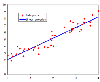
In statistics, linear regression is a model that estimates the linear relationship between a scalar response and one or more explanatory variables. A model with exactly one explanatory variable is a simple linear regression; a model with two or more explanatory variables is a multiple linear regression. This term is distinct from multivariate linear regression, which predicts multiple correlated dependent variables rather than a single dependent variable.
Functional regression is a version of regression analysis when responses or covariates include functional data. Functional regression models can be classified into four types depending on whether the responses or covariates are functional or scalar: (i) scalar responses with functional covariates, (ii) functional responses with scalar covariates, (iii) functional responses with functional covariates, and (iv) scalar or functional responses with functional and scalar covariates. In addition, functional regression models can be linear, partially linear, or nonlinear. In particular, functional polynomial models, functional single and multiple index models and functional additive models are three special cases of functional nonlinear models.
Nonlinear mixed-effects models constitute a class of statistical models generalizing linear mixed-effects models. Like linear mixed-effects models, they are particularly useful in settings where there are multiple measurements within the same statistical units or when there are dependencies between measurements on related statistical units. Nonlinear mixed-effects models are applied in many fields including medicine, public health, pharmacology, and ecology.


