Last updated • 14 min readFrom Wikipedia, The Free Encyclopedia
Branch of mathematics
Bass guitar time signal of open string A note (55 Hz). Fourier transform of bass guitar time signal of open string A note (55 Hz). Fourier analysis reveals the oscillatory components of signals and functions.
The subject of Fourier analysis encompasses a vast spectrum of mathematics. In the sciences and engineering, the process of decomposing a function into oscillatory components is often called Fourier analysis, while the operation of rebuilding the function from these pieces is known as Fourier synthesis. For example, determining what component frequencies are present in a musical note would involve computing the Fourier transform of a sampled musical note. One could then re-synthesize the same sound by including the frequency components as revealed in the Fourier analysis. In mathematics, the term Fourier analysis often refers to the study of both operations.
The decomposition process itself is called a Fourier transformation. Its output, the Fourier transform, is often given a more specific name, which depends on the domain and other properties of the function being transformed. Moreover, the original concept of Fourier analysis has been extended over time to apply to more and more abstract and general situations, and the general field is often known as harmonic analysis. Each transform used for analysis (see list of Fourier-related transforms) has a corresponding inverse transform that can be used for synthesis.
To use Fourier analysis, data must be equally spaced. Different approaches have been developed for analyzing unequally spaced data, notably the least-squares spectral analysis (LSSA) methods that use a least squares fit of sinusoids to data samples, similar to Fourier analysis.[2][3] Fourier analysis, the most used spectral method in science, generally boosts long-periodic noise in long gapped records; LSSA mitigates such problems.[4]
By the convolution theorem, Fourier transforms turn the complicated convolution operation into simple multiplication, which means that they provide an efficient way to compute convolution-based operations such as signal filtering, polynomial multiplication, and multiplying large numbers.[7]
The discrete version of the Fourier transform (see below) can be evaluated quickly on computers using fast Fourier transform (FFT) algorithms.[8]
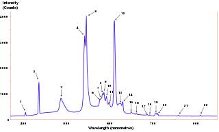
In forensics, laboratory infrared spectrophotometers use Fourier transform analysis for measuring the wavelengths of light at which a material will absorb in the infrared spectrum. The FT method is used to decode the measured signals and record the wavelength data. And by using a computer, these Fourier calculations are rapidly carried out, so that in a matter of seconds, a computer-operated FT-IR instrument can produce an infrared absorption pattern comparable to that of a prism instrument.[9]
Fourier transformation is also useful as a compact representation of a signal. For example, JPEG compression uses a variant of the Fourier transformation (discrete cosine transform) of small square pieces of a digital image. The Fourier components of each square are rounded to lower arithmetic precision, and weak components are eliminated, so that the remaining components can be stored very compactly. In image reconstruction, each image square is reassembled from the preserved approximate Fourier-transformed components, which are then inverse-transformed to produce an approximation of the original image.
When a function is a function of time and represents a physical signal, the transform has a standard interpretation as the frequency spectrum of the signal. The magnitude of the resulting complex-valued function at frequency represents the amplitude of a frequency component whose initial phase is given by the angle of (polar coordinates).
Fourier transforms are not limited to functions of time, and temporal frequencies. They can equally be applied to analyze spatial frequencies, and indeed for nearly any function domain. This justifies their use in such diverse branches as image processing, heat conduction, and automatic control.
When processing signals, such as audio, radio waves, light waves, seismic waves, and even images, Fourier analysis can isolate narrowband components of a compound waveform, concentrating them for easier detection or removal. A large family of signal processing techniques consist of Fourier-transforming a signal, manipulating the Fourier-transformed data in a simple way, and reversing the transformation.[10]
Generation of sound spectrograms used to analyze sounds;
Passive sonar used to classify targets based on machinery noise.
Variants of Fourier analysis
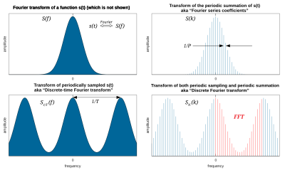
A Fourier transform and 3 variations caused by periodic sampling (at interval ) and/or periodic summation (at interval ) of the underlying time-domain function. The relative computational ease of the DFT sequence and the insight it gives into make it a popular analysis tool.
Most often, the unqualified term Fourier transform refers to the transform of functions of a continuous real argument, and it produces a continuous function of frequency, known as a frequency distribution. One function is transformed into another, and the operation is reversible. When the domain of the input (initial) function is time (), and the domain of the output (final) function is ordinary frequency, the transform of function at frequency is given by the complex number:
Evaluating this quantity for all values of produces the frequency-domain function. Then can be represented as a recombination of complex exponentials of all possible frequencies:
which is the inverse transform formula. The complex number, conveys both amplitude and phase of frequency
The Fourier transform of a periodic function, with period becomes a Dirac comb function, modulated by a sequence of complex coefficients:
(where is the integral over any interval of length ).
The inverse transform, known as Fourier series, is a representation of in terms of a summation of a potentially infinite number of harmonically related sinusoids or complex exponential functions, each with an amplitude and phase specified by one of the coefficients:
Note that any whose transform has the same discrete sample values can be used in the periodic summation. A sufficient condition for recovering (and therefore ) from just these samples (i.e. from the Fourier series) is that the non-zero portion of be confined to a known interval of duration which is the frequency domain dual of the Nyquist–Shannon sampling theorem.
See Fourier series for more information, including the historical development.
The DTFT is the mathematical dual of the time-domain Fourier series. Thus, a convergent periodic summation in the frequency domain can be represented by a Fourier series, whose coefficients are samples of a related continuous time function:
which is known as the DTFT. Thus the DTFT of the sequence is also the Fourier transform of the modulated Dirac comb function.[upper-alpha 2]
The Fourier series coefficients (and inverse transform), are defined by:
Parameter corresponds to the sampling interval, and this Fourier series can now be recognized as a form of the Poisson summation formula. Thus we have the important result that when a discrete data sequence, is proportional to samples of an underlying continuous function, one can observe a periodic summation of the continuous Fourier transform, Note that any with the same discrete sample values produces the same DTFT. But under certain idealized conditions one can theoretically recover and exactly. A sufficient condition for perfect recovery is that the non-zero portion of be confined to a known frequency interval of width When that interval is the applicable reconstruction formula is the Whittaker–Shannon interpolation formula. This is a cornerstone in the foundation of digital signal processing.
Another reason to be interested in is that it often provides insight into the amount of aliasing caused by the sampling process.
Applications of the DTFT are not limited to sampled functions. See Discrete-time Fourier transform for more information on this and other topics, including:
Similar to a Fourier series, the DTFT of a periodic sequence, with period , becomes a Dirac comb function, modulated by a sequence of complex coefficients (see DTFT §Periodic data):
(where is the sum over any sequence of length )
The sequence is customarily known as the DFT of one cycle of It is also -periodic, so it is never necessary to compute more than coefficients. The inverse transform, also known as a discrete Fourier series, is given by:
the coefficients are samples of at discrete intervals of :
Conversely, when one wants to compute an arbitrary number of discrete samples of one cycle of a continuous DTFT, it can be done by computing the relatively simple DFT of as defined above. In most cases, is chosen equal to the length of the non-zero portion of Increasing known as zero-padding or interpolation, results in more closely spaced samples of one cycle of Decreasing causes overlap (adding) in the time-domain (analogous to aliasing), which corresponds to decimation in the frequency domain. (see Discrete-time Fourier transform §L=N×I) In most cases of practical interest, the sequence represents a longer sequence that was truncated by the application of a finite-length window function or FIR filter array.
The DFT can be computed using a fast Fourier transform (FFT) algorithm, which makes it a practical and important transformation on computers.
For periodic functions, both the Fourier transform and the DTFT comprise only a discrete set of frequency components (Fourier series), and the transforms diverge at those frequencies. One common practice (not discussed above) is to handle that divergence via Dirac delta and Dirac comb functions. But the same spectral information can be discerned from just one cycle of the periodic function, since all the other cycles are identical. Similarly, finite-duration functions can be represented as a Fourier series, with no actual loss of information except that the periodicity of the inverse transform is a mere artifact.
It is common in practice for the duration of s(•) to be limited to the period, P or N. But these formulas do not require that condition.
transforms (continuous-time)
Continuous frequency
Discrete frequencies
Transform
Inverse
transforms (discrete-time)
Continuous frequency
Discrete frequencies
Transform
Inverse
Symmetry properties
When the real and imaginary parts of a complex function are decomposed into their even and odd parts, there are four components, denoted below by the subscripts RE, RO, IE, and IO. And there is a one-to-one mapping between the four components of a complex time function and the four components of its complex frequency transform:[11]
From this, various relationships are apparent, for example:
The transform of a real-valued function is the conjugate symmetric function Conversely, a conjugate symmetric transform implies a real-valued time-domain.
The transform of an imaginary-valued function is the conjugate antisymmetric function and the converse is true.
The transform of a conjugate symmetric function is the real-valued function and the converse is true.
The transform of a conjugate antisymmetric function is the imaginary-valued function and the converse is true.
In modern times, variants of the discrete Fourier transform were used by Alexis Clairaut in 1754 to compute an orbit,[16] which has been described as the first formula for the DFT,[17] and in 1759 by Joseph Louis Lagrange, in computing the coefficients of a trigonometric series for a vibrating string.[17] Technically, Clairaut's work was a cosine-only series (a form of discrete cosine transform), while Lagrange's work was a sine-only series (a form of discrete sine transform); a true cosine+sine DFT was used by Gauss in 1805 for trigonometric interpolation of asteroid orbits.[18] Euler and Lagrange both discretized the vibrating string problem, using what would today be called samples.[17]
An early modern development toward Fourier analysis was the 1770 paper Réflexions sur la résolution algébrique des équations by Lagrange, which in the method of Lagrange resolvents used a complex Fourier decomposition to study the solution of a cubic:[19] Lagrange transformed the roots into the resolvents:
where ζ is a cubic root of unity, which is the DFT of order 3.
Historians are divided as to how much to credit Lagrange and others for the development of Fourier theory:Daniel Bernoulli and Leonhard Euler had introduced trigonometric representations of functions, and Lagrange had given the Fourier series solution to the wave equation, so Fourier's contribution was mainly the bold claim that an arbitrary function could be represented by a Fourier series.[17]
The first fast Fourier transform (FFT) algorithm for the DFT was discovered around 1805 by Carl Friedrich Gauss when interpolating measurements of the orbit of the asteroids Juno and Pallas, although that particular FFT algorithm is more often attributed to its modern rediscoverers Cooley and Tukey.[18][16]
In signal processing terms, a function (of time) is a representation of a signal with perfect time resolution, but no frequency information, while the Fourier transform has perfect frequency resolution, but no time information.
Fourier transforms on arbitrary locally compact abelian topological groups
The Fourier variants can also be generalized to Fourier transforms on arbitrary locally compactAbeliantopological groups, which are studied in harmonic analysis; there, the Fourier transform takes functions on a group to functions on the dual group. This treatment also allows a general formulation of the convolution theorem, which relates Fourier transforms and convolutions. See also the Pontryagin duality for the generalized underpinnings of the Fourier transform.
More specific, Fourier analysis can be done on cosets,[21] even discrete cosets.
Consequently, a common practice is to model "sampling" as a multiplication by the Dirac comb function, which of course is only "possible" in a purely mathematical sense.
Related Research Articles
In mathematics, the discrete Fourier transform (DFT) converts a finite sequence of equally-spaced samples of a function into a same-length sequence of equally-spaced samples of the discrete-time Fourier transform (DTFT), which is a complex-valued function of frequency. The interval at which the DTFT is sampled is the reciprocal of the duration of the input sequence. An inverse DFT (IDFT) is a Fourier series, using the DTFT samples as coefficients of complex sinusoids at the corresponding DTFT frequencies. It has the same sample-values as the original input sequence. The DFT is therefore said to be a frequency domain representation of the original input sequence. If the original sequence spans all the non-zero values of a function, its DTFT is continuous, and the DFT provides discrete samples of one cycle. If the original sequence is one cycle of a periodic function, the DFT provides all the non-zero values of one DTFT cycle.
In physics, engineering and mathematics, the Fourier transform (FT) is an integral transform that takes a function as input and outputs another function that describes the extent to which various frequencies are present in the original function. The output of the transform is a complex-valued function of frequency. The term Fourier transform refers to both this complex-valued function and the mathematical operation. When a distinction needs to be made, the output of the operation is sometimes called the frequency domain representation of the original function. The Fourier transform is analogous to decomposing the sound of a musical chord into the intensities of its constituent pitches.
In mathematics, the convolution theorem states that under suitable conditions the Fourier transform of a convolution of two functions is the product of their Fourier transforms. More generally, convolution in one domain equals point-wise multiplication in the other domain. Other versions of the convolution theorem are applicable to various Fourier-related transforms.
A Fourier series is an expansion of a periodic function into a sum of trigonometric functions. The Fourier series is an example of a trigonometric series, but not all trigonometric series are Fourier series. By expressing a function as a sum of sines and cosines, many problems involving the function become easier to analyze because trigonometric functions are well understood. For example, Fourier series were first used by Joseph Fourier to find solutions to the heat equation. This application is possible because the derivatives of trigonometric functions fall into simple patterns. Fourier series cannot be used to approximate arbitrary functions, because most functions have infinitely many terms in their Fourier series, and the series do not always converge. Well-behaved functions, for example smooth functions, have Fourier series that converge to the original function. The coefficients of the Fourier series are determined by integrals of the function multiplied by trigonometric functions, described in Common forms of the Fourier series below.
In mathematics and signal processing, the Z-transform converts a discrete-time signal, which is a sequence of real or complex numbers, into a complex valued frequency-domain representation.
In signal processing, the power spectrum of a continuous time signal describes the distribution of power into frequency components composing that signal. According to Fourier analysis, any physical signal can be decomposed into a number of discrete frequencies, or a spectrum of frequencies over a continuous range. The statistical average of any sort of signal as analyzed in terms of its frequency content, is called its spectrum.
In mathematics, the Gibbs phenomenon is the oscillatory behavior of the Fourier series of a piecewise continuously differentiable periodic function around a jump discontinuity. The th partial Fourier series of the function produces large peaks around the jump which overshoot and undershoot the function values. As more sinusoids are used, this approximation error approaches a limit of about 9% of the jump, though the infinite Fourier series sum does eventually converge almost everywhere except points of discontinuity.
In signal processing, a finite impulse response (FIR) filter is a filter whose impulse response is of finite duration, because it settles to zero in finite time. This is in contrast to infinite impulse response (IIR) filters, which may have internal feedback and may continue to respond indefinitely.
In signal processing, a periodogram is an estimate of the spectral density of a signal. The term was coined by Arthur Schuster in 1898. Today, the periodogram is a component of more sophisticated methods. It is the most common tool for examining the amplitude vs frequency characteristics of FIR filters and window functions. FFT spectrum analyzers are also implemented as a time-sequence of periodograms.
In mathematics, the Poisson summation formula is an equation that relates the Fourier series coefficients of the periodic summation of a function to values of the function's continuous Fourier transform. Consequently, the periodic summation of a function is completely defined by discrete samples of the original function's Fourier transform. And conversely, the periodic summation of a function's Fourier transform is completely defined by discrete samples of the original function. The Poisson summation formula was discovered by Siméon Denis Poisson and is sometimes called Poisson resummation.
In mathematics and signal processing, the Hilbert transform is a specific singular integral that takes a function, u(t) of a real variable and produces another function of a real variable H(u)(t). The Hilbert transform is given by the Cauchy principal value of the convolution with the function (see § Definition). The Hilbert transform has a particularly simple representation in the frequency domain: It imparts a phase shift of ±90° (π/2 radians) to every frequency component of a function, the sign of the shift depending on the sign of the frequency (see § Relationship with the Fourier transform). The Hilbert transform is important in signal processing, where it is a component of the analytic representation of a real-valued signal u(t). The Hilbert transform was first introduced by David Hilbert in this setting, to solve a special case of the Riemann–Hilbert problem for analytic functions.
In mathematics, Parseval's theorem usually refers to the result that the Fourier transform is unitary; loosely, that the sum of the square of a function is equal to the sum of the square of its transform. It originates from a 1799 theorem about series by Marc-Antoine Parseval, which was later applied to the Fourier series. It is also known as Rayleigh's energy theorem, or Rayleigh's identity, after John William Strutt, Lord Rayleigh.
In mathematics, the discrete-time Fourier transform (DTFT) is a form of Fourier analysis that is applicable to a sequence of discrete values.
In mathematics, a Dirac comb is a periodic function with the formula :=\sum _{k=-\infty }^{\infty }\delta (t-kT)} for some given period . Here t is a real variable and the sum extends over all integers k. The Dirac delta function and the Dirac comb are tempered distributions. The graph of the function resembles a comb, hence its name and the use of the comb-like Cyrillic letter sha (Ш) to denote the function.
In digital signal processing, downsampling, compression, and decimation are terms associated with the process of resampling in a multi-rate digital signal processing system. Both downsampling and decimation can be synonymous with compression, or they can describe an entire process of bandwidth reduction (filtering) and sample-rate reduction. When the process is performed on a sequence of samples of a signal or a continuous function, it produces an approximation of the sequence that would have been obtained by sampling the signal at a lower rate.
The Hann function is named after the Austrian meteorologist Julius von Hann. It is a window function used to perform Hann smoothing. The function, with length and amplitude is given by:
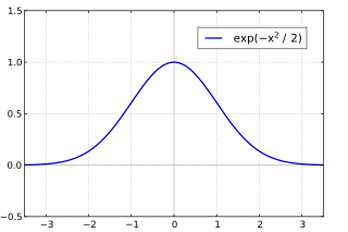
The Gabor transform, named after Dennis Gabor, is a special case of the short-time Fourier transform. It is used to determine the sinusoidal frequency and phase content of local sections of a signal as it changes over time. The function to be transformed is first multiplied by a Gaussian function, which can be regarded as a window function, and the resulting function is then transformed with a Fourier transform to derive the time-frequency analysis. The window function means that the signal near the time being analyzed will have higher weight. The Gabor transform of a signal x(t) is defined by this formula:
In statistical signal processing, the goal of spectral density estimation (SDE) or simply spectral estimation is to estimate the spectral density of a signal from a sequence of time samples of the signal. Intuitively speaking, the spectral density characterizes the frequency content of the signal. One purpose of estimating the spectral density is to detect any periodicities in the data, by observing peaks at the frequencies corresponding to these periodicities.
In digital signal processing, a discrete Fourier series (DFS) is a Fourier series whose sinusoidal components are functions of discrete time instead of continuous time. A specific example is the inverse discrete Fourier transform.
In mathematical analysis and applications, multidimensional transforms are used to analyze the frequency content of signals in a domain of two or more dimensions.
1 2 Heideman, M.T.; Johnson, D. H.; Burrus, C. S. (1984). "Gauss and the history of the fast Fourier transform". IEEE ASSP Magazine. 1 (4): 14–21. doi:10.1109/MASSP.1984.1162257. S2CID10032502.
This page is based on this Wikipedia article Text is available under the CC BY-SA 4.0 license; additional terms may apply. Images, videos and audio are available under their respective licenses.