Numerical analysis

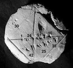
Babylonian clay tablet YBC 7289 (c. 1800–1600 BCE) with annotations. The approximation of the square root of 2 is four sexagesimal figures, which is about six decimal figures. 1 + 24/60 + 51/60 + 10/60 = 1.41421296...

Numerical analysis is the study of algorithms that use numerical approximation (as opposed to symbolic manipulations) for the problems of mathematical analysis (as distinguished from discrete mathematics). It is the study of numerical methods that attempt to find approximate solutions of problems rather than the exact ones. Numerical analysis finds application in all fields of engineering and the physical sciences, and in the 21st century also the life and social sciences like economics, medicine, business and even the arts. Current growth in computing power has enabled the use of more complex numerical analysis, providing detailed and realistic mathematical models in science and engineering. Examples of numerical analysis include: ordinary differential equations as found in celestial mechanics (predicting the motions of planets, stars and galaxies), numerical linear algebra in data analysis, ^{[2] [3] [4]} and stochastic differential equations and Markov chains for simulating living cells in medicine and biology.

Before modern computers, numerical methods often relied on hand interpolation formulas, using data from large printed tables. Since the mid 20th century, computers calculate the required functions instead, but many of the same formulas continue to be used in software algorithms. ^[5]

The numerical point of view goes back to the earliest mathematical writings. A tablet from the Yale Babylonian Collection (YBC 7289), gives a sexagesimal numerical approximation of the square root of 2, the length of the diagonal in a unit square.

Numerical analysis continues this long tradition: rather than giving exact symbolic answers translated into digits and applicable only to real-world measurements, approximate solutions within specified error bounds are used.

Applications

The overall goal of the field of numerical analysis is the design and analysis of techniques to give approximate but accurate solutions to a wide variety of hard problems, many of which are infeasible to solve symbolically:

• Advanced numerical methods are essential in making numerical weather prediction feasible.
• Computing the trajectory of a spacecraft requires the accurate numerical solution of a system of ordinary differential equations.
• Car companies can improve the crash safety of their vehicles by using computer simulations of car crashes. Such simulations essentially consist of solving partial differential equations numerically.
• In the financial field, (private investment funds) and other financial institutions use quantitative finance tools from numerical analysis to attempt to calculate the value of stocks and derivatives more precisely than other market participants. ^[6]
• Airlines use sophisticated optimization algorithms to decide ticket prices, airplane and crew assignments and fuel needs. Historically, such algorithms were developed within the overlapping field of operations research.
• Insurance companies use numerical programs for actuarial analysis.

History

The field of numerical analysis predates the invention of modern computers by many centuries. Linear interpolation was already in use more than 2000 years ago. Many great mathematicians of the past were preoccupied by numerical analysis, ^[5] as is obvious from the names of important algorithms like Newton's method, Lagrange interpolation polynomial, Gaussian elimination, or Euler's method. The origins of modern numerical analysis are often linked to a 1947 paper by John von Neumann and Herman Goldstine, ^{[7] [8]} but others consider modern numerical analysis to go back to work by E. T. Whittaker in 1912. ^[7]

NIST publication

To facilitate computations by hand, large books were produced with formulas and tables of data such as interpolation points and function coefficients. Using these tables, often calculated out to 16 decimal places or more for some functions, one could look up values to plug into the formulas given and achieve very good numerical estimates of some functions. The canonical work in the field is the NIST publication edited by Abramowitz and Stegun, a 1000-plus page book of a very large number of commonly used formulas and functions and their values at many points. The function values are no longer very useful when a computer is available, but the large listing of formulas can still be very handy.

The mechanical calculator was also developed as a tool for hand computation. These calculators evolved into electronic computers in the 1940s, and it was then found that these computers were also useful for administrative purposes. But the invention of the computer also influenced the field of numerical analysis, ^[5] since now longer and more complicated calculations could be done.

The Leslie Fox Prize for Numerical Analysis was initiated in 1985 by the Institute of Mathematics and its Applications.

Key concepts

Direct and iterative methods

Direct methods compute the solution to a problem in a finite number of steps. These methods would give the precise answer if they were performed in infinite precision arithmetic. Examples include Gaussian elimination, the QR factorization method for solving systems of linear equations, and the simplex method of linear programming. In practice, finite precision is used and the result is an approximation of the true solution (assuming stability).

In contrast to direct methods, iterative methods are not expected to terminate in a finite number of steps, even if infinite precision were possible. Starting from an initial guess, iterative methods form successive approximations that converge to the exact solution only in the limit. A convergence test, often involving the residual, is specified in order to decide when a sufficiently accurate solution has (hopefully) been found. Even using infinite precision arithmetic these methods would not reach the solution within a finite number of steps (in general). Examples include Newton's method, the bisection method, and Jacobi iteration. In computational matrix algebra, iterative methods are generally needed for large problems. ^{[9] [10] [11] [12]}

Iterative methods are more common than direct methods in numerical analysis. Some methods are direct in principle but are usually used as though they were not, e.g. GMRES and the conjugate gradient method. For these methods the number of steps needed to obtain the exact solution is so large that an approximation is accepted in the same manner as for an iterative method.

As an example, consider the problem of solving

3x³ + 4 = 28

for the unknown quantity x.

Direct method

	3x3 + 4 = 28.
Subtract 4	3x3 = 24.
Divide by 3	x3 =  8.
Take cube roots	x =  2.

For the iterative method, apply the bisection method to f(x) = 3x³− 24. The initial values are a = 0, b = 3, f(a) = −24, f(b) = 57.

Iterative method

a	b	mid	f(mid)
0	3	1.5	−13.875
1.5	3	2.25	10.17...
1.5	2.25	1.875	−4.22...
1.875	2.25	2.0625	2.32...

From this table it can be concluded that the solution is between 1.875 and 2.0625. The algorithm might return any number in that range with an error less than 0.2.

Conditioning

Ill-conditioned problem: Take the function f(x) = 1/(x − 1). Note that f(1.1) = 10 and f(1.001) = 1000: a change in x of less than 0.1 turns into a change in f(x) of nearly 1000. Evaluating f(x) near x = 1 is an ill-conditioned problem.

Well-conditioned problem: By contrast, evaluating the same function f(x) = 1/(x − 1) near x = 10 is a well-conditioned problem. For instance, f(10) = 1/9 ≈ 0.111 and f(11) = 0.1: a modest change in x leads to a modest change in f(x).

Discretization

Furthermore, continuous problems must sometimes be replaced by a discrete problem whose solution is known to approximate that of the continuous problem; this process is called 'discretization'. For example, the solution of a differential equation is a function. This function must be represented by a finite amount of data, for instance by its value at a finite number of points at its domain, even though this domain is a continuum.

Generation and propagation of errors

Further information: Error propagation

The study of errors forms an important part of numerical analysis. There are several ways in which error can be introduced in the solution of the problem.

Round-off

Round-off errors arise because it is impossible to represent all real numbers exactly on a machine with finite memory (which is what all practical digital computers are).

Truncation and discretization error

Truncation errors are committed when an iterative method is terminated or a mathematical procedure is approximated and the approximate solution differs from the exact solution. Similarly, discretization induces a discretization error because the solution of the discrete problem does not coincide with the solution of the continuous problem. In the example above to compute the solution of ${\displaystyle 3x^{3}+4=28}$, after ten iterations, the calculated root is roughly 1.99. Therefore, the truncation error is roughly 0.01.

Once an error is generated, it propagates through the calculation. For example, the operation + on a computer is inexact. A calculation of the type ⁠${\displaystyle a+b+c+d+e}$⁠ is even more inexact.

A truncation error is created when a mathematical procedure is approximated. To integrate a function exactly, an infinite sum of regions must be found, but numerically only a finite sum of regions can be found, and hence the approximation of the exact solution. Similarly, to differentiate a function, the differential element approaches zero, but numerically only a nonzero value of the differential element can be chosen.

Numerical stability and well-posed problems

An algorithm is called numerically stable if an error, whatever its cause, does not grow to be much larger during the calculation. ^[13] This happens if the problem is well-conditioned , meaning that the solution changes by only a small amount if the problem data are changed by a small amount. ^[13] To the contrary, if a problem is 'ill-conditioned', then any small error in the data will grow to be a large error. ^[13] Both the original problem and the algorithm used to solve that problem can be well-conditioned or ill-conditioned, and any combination is possible. So an algorithm that solves a well-conditioned problem may be either numerically stable or numerically unstable. An art of numerical analysis is to find a stable algorithm for solving a well-posed mathematical problem.

Areas of study

The field of numerical analysis includes many sub-disciplines. Some of the major ones are:

Computing values of functions

Interpolation: Observing that the temperature varies from 20 degrees Celsius at 1:00 to 14 degrees at 3:00, a linear interpolation of this data would conclude that it was 17 degrees at 2:00 and 18.5 degrees at 1:30pm. Extrapolation: If the gross domestic product of a country has been growing an average of 5% per year and was 100 billion last year, it might be extrapolated that it will be 105 billion this year. A line through 20 points Regression: In linear regression, given n points, a line is computed that passes as close as possible to those n points. How much for a glass of lemonade? Optimization: Suppose lemonade is sold at a lemonade stand, at $1.00 per glass, that 197 glasses of lemonade can be sold per day, and that for each increase of $0.01, one less glass of lemonade will be sold per day. If $1.485 could be charged, profit would be maximized, but due to the constraint of having to charge a whole-cent amount, charging $1.48 or $1.49 per glass will both yield the maximum income of $220.52 per day. Wind direction in blue, true trajectory in black, Euler method in red Differential equation: If 100 fans are set up to blow air from one end of the room to the other and then a feather is dropped into the wind, what happens? The feather will follow the air currents, which may be very complex. One approximation is to measure the speed at which the air is blowing near the feather every second, and advance the simulated feather as if it were moving in a straight line at that same speed for one second, before measuring the wind speed again. This is called the Euler method for solving an ordinary differential equation.

One of the simplest problems is the evaluation of a function at a given point. The most straightforward approach, of just plugging in the number in the formula is sometimes not very efficient. For polynomials, a better approach is using the Horner scheme, since it reduces the necessary number of multiplications and additions. Generally, it is important to estimate and control round-off errors arising from the use of floating-point arithmetic.

Interpolation, extrapolation, and regression

Interpolation solves the following problem: given the value of some unknown function at a number of points, what value does that function have at some other point between the given points?

Extrapolation is very similar to interpolation, except that now the value of the unknown function at a point which is outside the given points must be found. ^[14]

Regression is also similar, but it takes into account that the data are imprecise. Given some points, and a measurement of the value of some function at these points (with an error), the unknown function can be found. The least squares-method is one way to achieve this.

Solving equations and systems of equations

Another fundamental problem is computing the solution of some given equation. Two cases are commonly distinguished, depending on whether the equation is linear or not. For instance, the equation ${\displaystyle 2x+5=3}$ is linear while ${\displaystyle 2x^{2}+5=3}$ is not.

Much effort has been put in the development of methods for solving systems of linear equations. Standard direct methods, i.e., methods that use some matrix decomposition are Gaussian elimination, LU decomposition, Cholesky decomposition for symmetric (or hermitian) and positive-definite matrix, and QR decomposition for non-square matrices. Iterative methods such as the Jacobi method, Gauss–Seidel method, successive over-relaxation and conjugate gradient method ^[15] are usually preferred for large systems. General iterative methods can be developed using a matrix splitting.

Root-finding algorithms are used to solve nonlinear equations (they are so named since a root of a function is an argument for which the function yields zero). If the function is differentiable and the derivative is known, then Newton's method is a popular choice. ^{[16] [17]} Linearization is another technique for solving nonlinear equations.

Solving eigenvalue or singular value problems

Several important problems can be phrased in terms of eigenvalue decompositions or singular value decompositions. For instance, the spectral image compression algorithm ^[18] is based on the singular value decomposition. The corresponding tool in statistics is called principal component analysis.

Optimization

Main article: Mathematical optimization

Optimization problems ask for the point at which a given function is maximized (or minimized). Often, the point also has to satisfy some constraints.

The field of optimization is further split in several subfields, depending on the form of the objective function and the constraint. For instance, linear programming deals with the case that both the objective function and the constraints are linear. A famous method in linear programming is the simplex method.

The method of Lagrange multipliers can be used to reduce optimization problems with constraints to unconstrained optimization problems.

Evaluating integrals

Main article: Numerical integration

Numerical integration, in some instances also known as numerical quadrature, asks for the value of a definite integral. ^[19] Popular methods use one of the Newton–Cotes formulas (like the midpoint rule or Simpson's rule) or Gaussian quadrature. ^[20] These methods rely on a "divide and conquer" strategy, whereby an integral on a relatively large set is broken down into integrals on smaller sets. In higher dimensions, where these methods become prohibitively expensive in terms of computational effort, one may use Monte Carlo or quasi-Monte Carlo methods (see Monte Carlo integration ^[21] ), or, in modestly large dimensions, the method of sparse grids.

Differential equations

Main articles: Numerical ordinary differential equations and Numerical partial differential equations

Numerical analysis is also concerned with computing (in an approximate way) the solution of differential equations, both ordinary differential equations and partial differential equations. ^[22]

Partial differential equations are solved by first discretizing the equation, bringing it into a finite-dimensional subspace. ^[23] This can be done by a finite element method, ^{[24] [25] [26]} a finite difference method, ^[27] or (particularly in engineering) a finite volume method. ^[28] The theoretical justification of these methods often involves theorems from functional analysis. This reduces the problem to the solution of an algebraic equation.

Software

Main articles: List of numerical-analysis software and Comparison of numerical-analysis software

Since the late twentieth century, most algorithms are implemented in a variety of programming languages. The Netlib repository contains various collections of software routines for numerical problems, mostly in Fortran and C. Commercial products implementing many different numerical algorithms include the IMSL and NAG libraries; a free-software alternative is the GNU Scientific Library.

Over the years the Royal Statistical Society published numerous algorithms in its Applied Statistics (code for these "AS" functions is here); ACM similarly, in its Transactions on Mathematical Software ("TOMS" code is here). The Naval Surface Warfare Center several times published its Library of Mathematics Subroutines (code here).

There are several popular numerical computing applications such as MATLAB, ^{[29] [30] [31]} TK Solver, S-PLUS, and IDL ^[32] as well as free and open-source alternatives such as FreeMat, Scilab, ^{[33] [34]} GNU Octave (similar to Matlab), and IT++ (a C++ library). There are also programming languages such as R ^[35] (similar to S-PLUS), Julia, ^[36] and Python with libraries such as NumPy, SciPy ^{[37] [38] [39]} and SymPy. Performance varies widely: while vector and matrix operations are usually fast, scalar loops may vary in speed by more than an order of magnitude. ^{[40] [41]}

Many computer algebra systems such as Mathematica also benefit from the availability of arbitrary-precision arithmetic which can provide more accurate results. ^{[42] [43] [44] [45]}

Also, any spreadsheet software can be used to solve simple problems relating to numerical analysis. Excel, for example, has hundreds of available functions, including for matrices, which may be used in conjunction with its built in "solver".

See also

• Category:Numerical analysts
• Analysis of algorithms
• Approximation theory
• Computational science
• Computational physics
• Gordon Bell Prize
• Interval arithmetic
• List of numerical analysis topics
• Local linearization method
• Numerical differentiation
• Numerical Recipes
• Probabilistic numerics
• Symbolic-numeric computation
• Validated numerics

References

Citations

1. "Photograph, illustration, and description of the root(2) tablet from the Yale Babylonian Collection". Archived from the original on 13 August 2012. Retrieved 2 October 2006.
2. Demmel, J.W. (1997). Applied numerical linear algebra. SIAM. doi:10.1137/1.9781611971446. ISBN   978-1-61197-144-6.
3. Ciarlet, P.G.; Miara, B.; Thomas, J.M. (1989). Introduction to numerical linear algebra and optimization. Cambridge University Press. ISBN   9780521327886. OCLC   877155729.
4. Trefethen, Lloyd; Bau III, David (1997). Numerical Linear Algebra. SIAM. ISBN   978-0-89871-361-9.
5. Brezinski, C.; Wuytack, L. (2012). Numerical analysis: Historical developments in the 20th century. Elsevier. ISBN   978-0-444-59858-5.
6. Stephen Blyth. "An Introduction to Quantitative Finance". 2013. page VII.
7. Watson, G.A. (2010). "The history and development of numerical analysis in Scotland: a personal perspective" (PDF). The Birth of Numerical Analysis. World Scientific. pp. 161–177. ISBN   9789814469456.
8. Bultheel, Adhemar; Cools, Ronald, eds. (2010). The Birth of Numerical Analysis. Vol. 10. World Scientific. ISBN   978-981-283-625-0.
9. Saad, Y. (2003). Iterative methods for sparse linear systems. SIAM. ISBN   978-0-89871-534-7.
10. Hageman, L.A.; Young, D.M. (2012). Applied iterative methods (2nd ed.). Courier Corporation. ISBN   978-0-8284-0312-2.
11. Traub, J.F. (1982). Iterative methods for the solution of equations (2nd ed.). American Mathematical Society. ISBN   978-0-8284-0312-2.
12. Greenbaum, A. (1997). Iterative methods for solving linear systems. SIAM. ISBN   978-0-89871-396-1.
13. Higham 2002
14. Brezinski, C.; Zaglia, M.R. (2013). Extrapolation methods: theory and practice. Elsevier. ISBN   978-0-08-050622-7.
15. Hestenes, Magnus R.; Stiefel, Eduard (December 1952). "Methods of Conjugate Gradients for Solving Linear Systems" (PDF). Journal of Research of the National Bureau of Standards. 49 (6): 409–. doi:10.6028/jres.049.044.
16. Ezquerro Fernández, J.A.; Hernández Verón, M.Á. (2017). Newton's method: An updated approach of Kantorovich's theory. Birkhäuser. ISBN   978-3-319-55976-6.
17. Deuflhard, Peter (2006). Newton Methods for Nonlinear Problems. Affine Invariance and Adaptive Algorithms. Computational Mathematics. Vol. 35 (2nd ed.). Springer. ISBN   978-3-540-21099-3.
18. Ogden, C.J.; Huff, T. (1997). "The Singular Value Decomposition and Its Applications in Image Compression" (PDF). Math 45. College of the Redwoods. Archived from the original (PDF) on 25 September 2006.
19. Davis, P.J.; Rabinowitz, P. (2007). Methods of numerical integration. Courier Corporation. ISBN   978-0-486-45339-2.
20. Weisstein, Eric W. "Gaussian Quadrature". MathWorld .
21. Geweke, John (1996). "15. Monte carlo simulation and numerical integration". Handbook of Computational Economics. Vol. 1. Elsevier. pp. 731–800. doi:10.1016/S1574-0021(96)01017-9. ISBN   9780444898579.
22. Iserles, A. (2009). A first course in the numerical analysis of differential equations (2nd ed.). Cambridge University Press. ISBN   978-0-521-73490-5.
23. Ames, W.F. (2014). Numerical methods for partial differential equations (3rd ed.). Academic Press. ISBN   978-0-08-057130-0.
24. Johnson, C. (2012). Numerical solution of partial differential equations by the finite element method. Courier Corporation. ISBN   978-0-486-46900-3.
25. Brenner, S.; Scott, R. (2013). The mathematical theory of finite element methods (2nd ed.). Springer. ISBN   978-1-4757-3658-8.
26. Strang, G.; Fix, G.J. (2018) [1973]. An analysis of the finite element method (2nd ed.). Wellesley-Cambridge Press. ISBN   9780980232783. OCLC   1145780513.
27. Strikwerda, J.C. (2004). Finite difference schemes and partial differential equations (2nd ed.). SIAM. ISBN   978-0-89871-793-8.
28. LeVeque, Randall (2002). Finite Volume Methods for Hyperbolic Problems. Cambridge University Press. ISBN   978-1-139-43418-8.
29. Quarteroni, A.; Saleri, F.; Gervasio, P. (2014). Scientific computing with MATLAB and Octave (4th ed.). Springer. ISBN   978-3-642-45367-0.
30. Gander, W.; Hrebicek, J., eds. (2011). Solving problems in scientific computing using Maple and Matlab®. Springer. ISBN   978-3-642-18873-2.
31. Barnes, B.; Fulford, G.R. (2011). Mathematical modelling with case studies: a differential equations approach using Maple and MATLAB (2nd ed.). CRC Press. ISBN   978-1-4200-8350-7. OCLC   1058138488.
32. Gumley, L.E. (2001). Practical IDL programming. Elsevier. ISBN   978-0-08-051444-4.
33. Bunks, C.; Chancelier, J.P.; Delebecque, F.; Goursat, M.; Nikoukhah, R.; Steer, S. (2012). Engineering and scientific computing with Scilab. Springer. ISBN   978-1-4612-7204-5.
34. Thanki, R.M.; Kothari, A.M. (2019). Digital image processing using SCILAB. Springer. ISBN   978-3-319-89533-8.
35. Ihaka, R.; Gentleman, R. (1996). "R: a language for data analysis and graphics" (PDF). Journal of Computational and Graphical Statistics. 5 (3): 299–314. doi:10.1080/10618600.1996.10474713. S2CID   60206680.
36. Bezanson, Jeff; Edelman, Alan; Karpinski, Stefan; Shah, Viral B. (1 January 2017). "Julia: A Fresh Approach to Numerical Computing". SIAM Review. 59 (1): 65–98. arXiv: 1411.1607 . doi:10.1137/141000671. hdl: 1721.1/110125 . ISSN   0036-1445. S2CID   13026838.
37. Jones, E., Oliphant, T., & Peterson, P. (2001). SciPy: Open source scientific tools for Python.
38. Bressert, E. (2012). SciPy and NumPy: an overview for developers. O'Reilly. ISBN   9781306810395.
39. Blanco-Silva, F.J. (2013). Learning SciPy for numerical and scientific computing. Packt. ISBN   9781782161639.
40. Speed comparison of various number crunching packages Archived 5 October 2006 at the Wayback Machine
41. Comparison of mathematical programs for data analysis Archived 18 May 2016 at the Portuguese Web Archive Stefan Steinhaus, ScientificWeb.com
42. Maeder, R.E. (1997). Programming in mathematica (3rd ed.). Addison-Wesley. ISBN   9780201854497. OCLC   1311056676.
43. Wolfram, Stephen (1999). The MATHEMATICA® book, version 4. Cambridge University Press. ISBN   9781579550042.
44. Shaw, W.T.; Tigg, J. (1993). Applied Mathematica: getting started, getting it done (PDF). Addison-Wesley. ISBN   978-0-201-54217-2. OCLC   28149048.
45. Marasco, A.; Romano, A. (2001). Scientific Computing with Mathematica: Mathematical Problems for Ordinary Differential Equations. Springer. ISBN   978-0-8176-4205-1.

Sources

• Golub, Gene H.; Charles F. Van Loan (1986). Matrix Computations (3rd ed.). Johns Hopkins University Press. ISBN   0-8018-5413-X.
• Ralston Anthony; Rabinowitz Philips (2001). A First Course in Numerical Analysis (2nd ed.). Dover publications. ISBN   978-0486414546.
• Higham, Nicholas J. (2002) [1996]. Accuracy and Stability of Numerical Algorithms . Society for Industrial and Applied Mathematics. ISBN   0-89871-355-2.
• Hildebrand, F. B. (1974). Introduction to Numerical Analysis (2nd ed.). McGraw-Hill. ISBN   0-07-028761-9.
• David Kincaid and Ward Cheney: Numerical Analysis : Mathematics of Scientific Computing, 3rd Ed., AMS, ISBN 978-0-8218-4788-6 (2002).
• Leader, Jeffery J. (2004). Numerical Analysis and Scientific Computation. Addison Wesley. ISBN   0-201-73499-0.
• Wilkinson, J.H. (1988) [1965]. The Algebraic Eigenvalue Problem . Clarendon Press. ISBN   978-0-19-853418-1.
• Kahan, W. (1972). A survey of error-analysis. Proc. IFIP Congress 71 in Ljubljana. Info. Processing 71. Vol. 2. North-Holland. pp. 1214–39. ISBN   978-0-7204-2063-0. OCLC   25116949. (examples of the importance of accurate arithmetic).
• Trefethen, Lloyd N. (2008). "IV.21 Numerical analysis" (PDF). In Leader, I.; Gowers, T.; Barrow-Green, J. (eds.). Princeton Companion of Mathematics. Princeton University Press. pp. 604–614. ISBN   978-0-691-11880-2.

External links

Journals

• Numerische Mathematik , volumes 1–..., Springer, 1959–
  • volumes 1–66, 1959–1994 (searchable; pages are images). (in English and German)
• Journal on Numerical Analysis (SINUM), volumes 1–..., SIAM, 1964–

Online texts

• "Numerical analysis", Encyclopedia of Mathematics , EMS Press, 2001 [1994]
• Numerical Recipes, William H. Press (free, downloadable previous editions)
• First Steps in Numerical Analysis (archived), R.J.Hosking, S.Joe, D.C.Joyce, and J.C.Turner
• CSEP (Computational Science Education Project), U.S. Department of Energy (archived 2017-08-01)
• Numerical Methods, ch 3. in the Digital Library of Mathematical Functions
• Numerical Interpolation, Differentiation and Integration, ch 25. in the Handbook of Mathematical Functions (Abramowitz and Stegun)

Online course material

• Numerical Methods (Archived 28 July 2009 at the Wayback Machine ), Stuart Dalziel University of Cambridge
• Lectures on Numerical Analysis, Dennis Deturck and Herbert S. Wilf University of Pennsylvania
• Numerical methods, John D. Fenton University of Karlsruhe
• Numerical Methods for Physicists, Anthony O’Hare Oxford University
• Lectures in Numerical Analysis (archived), R. Radok Mahidol University
• Introduction to Numerical Analysis for Engineering, Henrik Schmidt Massachusetts Institute of Technology
• Numerical Analysis for Engineering, D. W. Harder University of Waterloo
• Introduction to Numerical Analysis, Doron Levy University of Maryland
• Numerical Analysis - Numerical Methods (archived), John H. Mathews California State University Fullerton