Numerical differentiation

Finite difference estimation of derivative

In numerical analysis, numerical differentiation algorithms estimate the derivative of a mathematical function or function subroutine using values of the function and perhaps other knowledge about the function.

Finite differences

Further information: Finite differences

The simplest method is to use finite difference approximations.

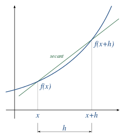
A simple two-point estimation is to compute the slope of a nearby secant line through the points (x, f(x)) and (x + h, f(x + h)). ^[1] Choosing a small number h, h represents a small change in x, and it can be either positive or negative. The slope of this line is $${\displaystyle {\frac {f(x+h)-f(x)}{h}}.}$$ This expression is Newton's difference quotient (also known as a first-order divided difference).

The slope of this secant line differs from the slope of the tangent line by an amount that is approximately proportional to h. As h approaches zero, the slope of the secant line approaches the slope of the tangent line. Therefore, the true derivative of f at x is the limit of the value of the difference quotient as the secant lines get closer and closer to being a tangent line: $${\displaystyle f'(x)=\lim _{h\to 0}{\frac {f(x+h)-f(x)}{h}}.}$$

Since immediately substituting 0 for h results in ${\displaystyle {\frac {0}{0}}}$ indeterminate form, calculating the derivative directly can be unintuitive.

Equivalently, the slope could be estimated by employing positions x − h and x.

Another two-point formula is to compute the slope of a nearby secant line through the points (x − h, f(x − h)) and (x + h, f(x + h)). The slope of this line is $${\displaystyle {\frac {f(x+h)-f(x-h)}{2h}}.}$$

This formula is known as the symmetric difference quotient. In this case the first-order errors cancel, so the slope of these secant lines differ from the slope of the tangent line by an amount that is approximately proportional to ${\displaystyle h^{2}}$. Hence for small values of h this is a more accurate approximation to the tangent line than the one-sided estimation. However, although the slope is being computed at x, the value of the function at x is not involved.

The estimation error is given by $${\displaystyle R={\frac {-f^{(3)}(c)}{6}}h^{2},}$$ where ${\displaystyle c}$ is some point between ${\displaystyle x-h}$ and ${\displaystyle x+h}$. This error does not include the rounding error due to numbers being represented and calculations being performed in limited precision.

The symmetric difference quotient is employed as the method of approximating the derivative in a number of calculators, including TI-82, TI-83, TI-84, TI-85, all of which use this method with h = 0.001. ^{[2] [3]}

Step size

See also: Adaptive step size

Example showing the difficulty of choosing h due to both rounding error and formula error

An important consideration in practice when the function is calculated using floating-point arithmetic of finite precision is the choice of step size, h. If chosen too small, the subtraction will yield a large rounding error. In fact, all the finite-difference formulae are ill-conditioned ^[4] and due to cancellation will produce a value of zero if h is small enough. ^[5] If too large, the calculation of the slope of the secant line will be more accurately calculated, but the estimate of the slope of the tangent by using the secant could be worse. ^[6]

For basic central differences, the optimal step is the cube-root of machine epsilon. ^[7] For the numerical derivative formula evaluated at x and x + h, a choice for h that is small without producing a large rounding error is ${\displaystyle {\sqrt {\varepsilon }}x}$ (though not when x = 0), where the machine epsilon ε is typically of the order of 2.2×10⁻¹⁶ for double precision. ^[8] A formula for h that balances the rounding error against the secant error for optimum accuracy is ^[9] $${\displaystyle h=2{\sqrt {\varepsilon \left|{\frac {f(x)}{f''(x)}}\right|}}}$$ (though not when ${\displaystyle f''(x)=0}$), and to employ it will require knowledge of the function.

For computer calculations the problems are exacerbated because, although x necessarily holds a representable floating-point number in some precision (32 or 64-bit, etc.), x + h almost certainly will not be exactly representable in that precision. This means that x + h will be changed (by rounding or truncation) to a nearby machine-representable number, with the consequence that (x + h) − x will not equal h; the two function evaluations will not be exactly h apart. In this regard, since most decimal fractions are recurring sequences in binary (just as 1/3 is in decimal) a seemingly round step such as h = 0.1 will not be a round number in binary; it is 0.000110011001100...₂ A possible approach is as follows:

h     := sqrt(eps) * x; xph   := x + h; dx    := xph - x; slope := (F(xph) - F(x)) / dx;

However, with computers, compiler optimization facilities may fail to attend to the details of actual computer arithmetic and instead apply the axioms of mathematics to deduce that dx and h are the same. With C and similar languages, a directive that xph is a volatile variable will prevent this.

Other methods

Higher-order methods

Further information: Finite difference coefficient

Higher-order methods for approximating the derivative, as well as methods for higher derivatives, exist.

Given below is the five-point method for the first derivative (five-point stencil in one dimension): ^[10] $${\displaystyle f'(x)={\frac {-f(x+2h)+8f(x+h)-8f(x-h)+f(x-2h)}{12h}}+{\frac {h^{4}}{30}}f^{(5)}(c),}$$ where ${\displaystyle c\in [x-2h,x+2h]}$.

For other stencil configurations and derivative orders, the Finite Difference Coefficients Calculator is a tool that can be used to generate derivative approximation methods for any stencil with any derivative order (provided a solution exists).

Higher derivatives

Using Newton's difference quotient, $${\displaystyle f'(x)=\lim _{h\to 0}{\frac {f(x+h)-f(x)}{h}}}$$ the following can be shown ^[11] (for n > 0): $${\displaystyle f^{(n)}(x)=\lim _{h\to 0}{\frac {1}{h^{n}}}\sum _{k=0}^{n}(-1)^{k+n}{\binom {n}{k}}f(x+kh)}$$

Complex-variable methods

The classical finite-difference approximations for numerical differentiation are ill-conditioned. However, if ${\displaystyle f}$ is a holomorphic function, real-valued on the real line, which can be evaluated at points in the complex plane near ${\displaystyle x}$, then there are stable methods. For example, ^[5] the first derivative can be calculated by the complex-step derivative formula: ^{[12] [13] [14]} $${\displaystyle f'(x)={\frac {\Im (f(x+\mathrm {i} h))}{h}}+O(h^{2}),\quad \mathrm {i^{2}}$$ :=-1.}

The recommended step size to obtain accurate derivatives for a range of conditions is ${\displaystyle h=10^{-200}}$. ^[6] This formula can be obtained by Taylor series expansion: $${\displaystyle f(x+\mathrm {i} h)=f(x)+\mathrm {i} hf'(x)-{\tfrac {1}{2!}}h^{2}f''(x)-{\tfrac {\mathrm {i} }{3!}}h^{3}f^{(3)}(x)+\cdots .}$$

The complex-step derivative formula is only valid for calculating first-order derivatives. A generalization of the above for calculating derivatives of any order employs multicomplex numbers, resulting in multicomplex derivatives. ^{[15] [16] [17]} $${\displaystyle f^{(n)}(x)\approx {\frac {{\mathcal {C}}_{n^{2}-1}^{(n)}(f(x+\mathrm {i} ^{(1)}h+\cdots +\mathrm {i} ^{(n)}h))}{h^{n}}}}$$ where the ${\displaystyle \mathrm {i} ^{(k)}}$ denote the multicomplex imaginary units; ${\displaystyle \mathrm {i} ^{(1)}\equiv \mathrm {i} }$. The ${\displaystyle {\mathcal {C}}_{k}^{(n)}}$ operator extracts the ${\displaystyle k}$th component of a multicomplex number of level ${\displaystyle n}$, e.g., ${\displaystyle {\mathcal {C}}_{0}^{(n)}}$ extracts the real component and ${\displaystyle {\mathcal {C}}_{n^{2}-1}^{(n)}}$ extracts the last, “most imaginary” component. The method can be applied to mixed derivatives, e.g. for a second-order derivative $${\displaystyle {\frac {\partial ^{2}f(x,y)}{\partial x\,\partial y}}\approx {\frac {{\mathcal {C}}_{3}^{(2)}(f(x+\mathrm {i} ^{(1)}h,y+\mathrm {i} ^{(2)}h))}{h^{2}}}}$$

A C++ implementation of multicomplex arithmetics is available. ^[18]

In general, derivatives of any order can be calculated using Cauchy's integral formula: ^[19] $${\displaystyle f^{(n)}(a)={\frac {n!}{2\pi i}}\oint _{\gamma }{\frac {f(z)}{(z-a)^{n+1}}}\,\mathrm {d} z,}$$ where the integration is done numerically.

Using complex variables for numerical differentiation was started by Lyness and Moler in 1967. ^[20] Their algorithm is applicable to higher-order derivatives.

A method based on numerical inversion of a complex Laplace transform was developed by Abate and Dubner. ^[21] An algorithm that can be used without requiring knowledge about the method or the character of the function was developed by Fornberg. ^[4]

Differential quadrature

Differential quadrature is the approximation of derivatives by using weighted sums of function values. ^{[22] [23]} Differential quadrature is of practical interest because its allows one to compute derivatives from noisy data. The name is in analogy with quadrature, meaning numerical integration, where weighted sums are used in methods such as Simpson's method or the Trapezoidal rule. There are various methods for determining the weight coefficients, for example, the Savitzky–Golay filter. Differential quadrature is used to solve partial differential equations. There are further methods for computing derivatives from noisy data. ^[24]

See also

• Automatic differentiation  – Numerical calculations carrying along derivatives
• Five-point stencil  – A point and its four nearest neighbors
• Savitzky-Golay filter  – Algorithm to smooth data pointsPages displaying short descriptions of redirect targets
• Numerical integration  – Methods of calculating definite integrals
• Numerical ordinary differential equations  – Methods used to find numerical solutions of ordinary differential equationsPages displaying short descriptions of redirect targets
• Numerical smoothing and differentiation  – Algorithm to smooth data pointsPages displaying short descriptions of redirect targets
• List of numerical-analysis software

References

1. Richard L. Burden, J. Douglas Faires (2000), Numerical Analysis, (7th Ed), Brooks/Cole. ISBN   0-534-38216-9.
2. Katherine Klippert Merseth (2003). Windows on Teaching Math: Cases of Middle and Secondary Classrooms . Teachers College Press. p.  34. ISBN   978-0-8077-4279-2.
3. Tamara Lefcourt Ruby; James Sellers; Lisa Korf; Jeremy Van Horn; Mike Munn (2014). Kaplan AP Calculus AB & BC 2015. Kaplan Publishing. p. 299. ISBN   978-1-61865-686-5.
4. Numerical Differentiation of Analytic Functions, B Fornberg – ACM Transactions on Mathematical Software (TOMS), 1981.
5. Using Complex Variables to Estimate Derivatives of Real Functions, W. Squire, G. Trapp – SIAM REVIEW, 1998.
6. Martins, Joaquim R. R. A.; Ning, Andrew (2021-10-01). Engineering Design Optimization (PDF). Cambridge University Press. ISBN   978-1108833417.
7. Sauer, Timothy (2012). Numerical Analysis. Pearson. p.248.
8. Following Numerical Recipes in C, Chapter 5.7.
9. p. 263.
10. Abramowitz & Stegun, Table 25.2.
11. Shilov, George. Elementary Real and Complex Analysis.
12. Martins, J. R. R. A.; Sturdza, P.; Alonso, J. J. (2003). "The Complex-Step Derivative Approximation". ACM Transactions on Mathematical Software. 29 (3): 245–262. CiteSeerX   10.1.1.141.8002 . doi:10.1145/838250.838251. S2CID   7022422.
13. Differentiation With(out) a Difference by Nicholas Higham
14. article from MathWorks blog, posted by Cleve Moler
15. "Archived copy" (PDF). Archived from the original (PDF) on 2014-01-09. Retrieved 2012-11-24.
16. Lantoine, G.; Russell, R. P.; Dargent, Th. (2012). "Using multicomplex variables for automatic computation of high-order derivatives". ACM Trans. Math. Softw. 38 (3): 1–21. doi:10.1145/2168773.2168774. S2CID   16253562.
17. Verheyleweghen, A. (2014). "Computation of higher-order derivatives using the multi-complex step method" (PDF).
18. Bell, I. H. (2019). "mcx (multicomplex algebra library)". GitHub .
19. Ablowitz, M. J., Fokas, A. S.,(2003). Complex variables: introduction and applications. Cambridge University Press. Check theorem 2.6.2
20. Lyness, J. N.; Moler, C. B. (1967). "Numerical differentiation of analytic functions". SIAM J. Numer. Anal. 4 (2): 202–210. Bibcode:1967SJNA....4..202L. doi:10.1137/0704019.
21. Abate, J; Dubner, H (March 1968). "A New Method for Generating Power Series Expansions of Functions". SIAM J. Numer. Anal. 5 (1): 102–112. Bibcode:1968SJNA....5..102A. doi:10.1137/0705008.
22. Differential Quadrature and Its Application in Engineering: Engineering Applications, Chang Shu, Springer, 2000, ISBN   978-1-85233-209-9.
23. Advanced Differential Quadrature Methods, Yingyan Zhang, CRC Press, 2009, ISBN   978-1-4200-8248-7.
24. Ahnert, Karsten; Abel, Markus (2007). "Numerical differentiation of experimental data: local versus global methods". Computer Physics Communications. 177 (10): 764–774. Bibcode:2007CoPhC.177..764A. CiteSeerX   10.1.1.752.3843 . doi:10.1016/j.cpc.2007.03.009. ISSN   0010-4655. S2CID   15129086.

External links

• Numerical Differentiation from wolfram.com
• NAG Library numerical differentiation routines
• Boost. Math numerical differentiation, including finite differencing and the complex step derivative
• Differentiation With(out) a Difference by Nicholas Higham, SIAM News.