Trapezoidal rule

Last updated
The function f(x) (in blue) is approximated by a linear function (in red). Trapezoidal rule illustration.svg
The function f(x) (in blue) is approximated by a linear function (in red).

In calculus, the trapezoidal rule (also known as the trapezoid rule or trapezium rule) [lower-alpha 1] is a technique for numerical integration, i.e., approximating the definite integral:

Contents

The trapezoidal rule works by approximating the region under the graph of the function as a trapezoid and calculating its area. It follows that

An animation that shows what the trapezoidal rule is and how the error in approximation decreases as the step size decreases WikiTrap.gif
An animation that shows what the trapezoidal rule is and how the error in approximation decreases as the step size decreases

The trapezoidal rule may be viewed as the result obtained by averaging the left and right Riemann sums, and is sometimes defined this way. The integral can be even better approximated by partitioning the integration interval, applying the trapezoidal rule to each subinterval, and summing the results. In practice, this "chained" (or "composite") trapezoidal rule is usually what is meant by "integrating with the trapezoidal rule". Let be a partition of such that and be the length of the -th subinterval (that is, ), then

When the partition has a regular spacing, as is often the case, that is, when all the have the same value the formula can be simplified for calculation efficiency by factoring out:.

The approximation becomes more accurate as the resolution of the partition increases (that is, for larger , all decrease).

As discussed below, it is also possible to place error bounds on the accuracy of the value of a definite integral estimated using a trapezoidal rule.

Illustration of "chained trapezoidal rule" used on an irregularly-spaced partition of
[
a
,
b
]
{\displaystyle [a,b]}
. Integration num trapezes notation.svg
Illustration of "chained trapezoidal rule" used on an irregularly-spaced partition of .

History

A 2016 Science paper reports that the trapezoid rule was in use in Babylon before 50 BCE for integrating the velocity of Jupiter along the ecliptic. [1]

Numerical implementation

Non-uniform grid

When the grid spacing is non-uniform, one can use the formula

wherein

Uniform grid

For a domain discretized into equally spaced panels, considerable simplification may occur. Let

the approximation to the integral becomes

Error analysis

An animation showing how the trapezoidal rule approximation improves with more strips for an interval with
a
=
2
{\displaystyle a=2}
and
b
=
8
{\displaystyle b=8}
. As the number of intervals
N
{\displaystyle N}
increases, so too does the accuracy of the result. Trapezium2.gif
An animation showing how the trapezoidal rule approximation improves with more strips for an interval with and . As the number of intervals increases, so too does the accuracy of the result.

The error of the composite trapezoidal rule is the difference between the value of the integral and the numerical result:

There exists a number ξ between a and b, such that [2]

It follows that if the integrand is concave up (and thus has a positive second derivative), then the error is negative and the trapezoidal rule overestimates the true value. This can also be seen from the geometric picture: the trapezoids include all of the area under the curve and extend over it. Similarly, a concave-down function yields an underestimate because area is unaccounted for under the curve, but none is counted above. If the interval of the integral being approximated includes an inflection point, the error is harder to identify.

An asymptotic error estimate for N → ∞ is given by

Further terms in this error estimate are given by the Euler–Maclaurin summation formula.

Several techniques can be used to analyze the error, including: [3]

  1. Fourier series
  2. Residue calculus
  3. Euler–Maclaurin summation formula [4] [5]
  4. Polynomial interpolation [6]

It is argued that the speed of convergence of the trapezoidal rule reflects and can be used as a definition of classes of smoothness of the functions. [7]

Proof

First suppose that and . Let

be the function such that is the error of the trapezoidal rule on one of the intervals, . Then

and

Now suppose that which holds if is sufficiently smooth. It then follows that

which is equivalent to , or

Since and ,

and

Using these results, we find

and

Letting we find

Summing all of the local error terms we find

But we also have

and

so that

Therefore the total error is bounded by

Periodic and peak functions

The trapezoidal rule converges rapidly for periodic functions. This is an easy consequence of the Euler-Maclaurin summation formula, which says that if is times continuously differentiable with period

where and is the periodic extension of the th Bernoulli polynomial. [8] Due to the periodicity, the derivatives at the endpoint cancel and we see that the error is .

A similar effect is available for peak-like functions, such as Gaussian, Exponentially modified Gaussian and other functions with derivatives at integration limits that can be neglected. [9] The evaluation of the full integral of a Gaussian function by trapezoidal rule with 1% accuracy can be made using just 4 points. [10] Simpson's rule requires 1.8 times more points to achieve the same accuracy. [10] [11]

Although some effort has been made to extend the Euler-Maclaurin summation formula to higher dimensions, [12] the most straightforward proof of the rapid convergence of the trapezoidal rule in higher dimensions is to reduce the problem to that of convergence of Fourier series. This line of reasoning shows that if is periodic on a -dimensional space with continuous derivatives, the speed of convergence is . For very large dimension, the shows that Monte-Carlo integration is most likely a better choice, but for 2 and 3 dimensions, equispaced sampling is efficient. This is exploited in computational solid state physics where equispaced sampling over primitive cells in the reciprocal lattice is known as Monkhorst-Pack integration. [13]

"Rough" functions

For functions that are not in C2, the error bound given above is not applicable. Still, error bounds for such rough functions can be derived, which typically show a slower convergence with the number of function evaluations than the behaviour given above. Interestingly, in this case the trapezoidal rule often has sharper bounds than Simpson's rule for the same number of function evaluations. [14]

Applicability and alternatives

The trapezoidal rule is one of a family of formulas for numerical integration called Newton–Cotes formulas, of which the midpoint rule is similar to the trapezoid rule. Simpson's rule is another member of the same family, and in general has faster convergence than the trapezoidal rule for functions which are twice continuously differentiable, though not in all specific cases. However, for various classes of rougher functions (ones with weaker smoothness conditions), the trapezoidal rule has faster convergence in general than Simpson's rule. [14]

Moreover, the trapezoidal rule tends to become extremely accurate when periodic functions are integrated over their periods, which can be analyzed in various ways. [7] [11] A similar effect is available for peak functions. [10] [11]

For non-periodic functions, however, methods with unequally spaced points such as Gaussian quadrature and Clenshaw–Curtis quadrature are generally far more accurate; Clenshaw–Curtis quadrature can be viewed as a change of variables to express arbitrary integrals in terms of periodic integrals, at which point the trapezoidal rule can be applied accurately.

Example

The following integral is given:

  1.  Use the composite trapezoidal rule to estimate the value of this integral. Use three segments.
  2.  Find the true error for part (a).
  3.  Find the absolute relative true error for part (a).

Solution

  1. The solution using the composite trapezoidal rule with 3 segments is applied as follows.

    Using the composite trapezoidal rule formula

  2. The exact value of the above integral can be found by integration by parts and is

    So the true error is

  3. The absolute relative true error is

See also

Notes

  1. See Trapezoid for more information on terminology.
  1. Ossendrijver, Mathieu (Jan 29, 2016). "Ancient Babylonian astronomers calculated Jupiter's position from the area under a time-velocity graph". Science. 351 (6272): 482–484. doi:10.1126/science.aad8085. PMID   26823423. S2CID   206644971.
  2. Atkinson (1989 , equation (5.1.7))
  3. ( Weideman 2002 , p. 23, section 2)
  4. Atkinson (1989 , equation (5.1.9))
  5. Atkinson (1989 , p. 285)
  6. Burden & Faires (2011 , p. 194)
  7. 1 2 ( Rahman & Schmeisser 1990 )
  8. Kress, Rainer (1998). Numerical Analysis, volume 181 of Graduate Texts in Mathematics. Springer-Verlag.
  9. Goodwin, E. T. (1949). "The evaluation of integrals of the form". Mathematical Proceedings of the Cambridge Philosophical Society. 45 (2): 241–245. doi:10.1017/S0305004100024786. ISSN   1469-8064.
  10. 1 2 3 Kalambet, Yuri; Kozmin, Yuri; Samokhin, Andrey (2018). "Comparison of integration rules in the case of very narrow chromatographic peaks". Chemometrics and Intelligent Laboratory Systems. 179: 22–30. doi:10.1016/j.chemolab.2018.06.001. ISSN   0169-7439.
  11. 1 2 3 ( Weideman 2002 )
  12. "Euler-Maclaurin Summation Formula for Multiple Sums". math.stackexchange.com.
  13. Thompson, Nick. "Numerical Integration over Brillouin Zones". bandgap.io. Retrieved 19 December 2017.
  14. 1 2 ( Cruz-Uribe & Neugebauer 2002 )

Related Research Articles

<span class="mw-page-title-main">Integral</span> Operation in mathematical calculus

In mathematics, an integral is the continuous analog of a sum, which is used to calculate areas, volumes, and their generalizations. Integration, the process of computing an integral, is one of the two fundamental operations of calculus, the other being differentiation. Integration was initially used to solve problems in mathematics and physics, such as finding the area under a curve, or determining displacement from velocity. Usage of integration expanded to a wide variety of scientific fields thereafter.

<span class="mw-page-title-main">Dirac delta function</span> Generalized function whose value is zero everywhere except at zero

In mathematical analysis, the Dirac delta function, also known as the unit impulse, is a generalized function on the real numbers, whose value is zero everywhere except at zero, and whose integral over the entire real line is equal to one. Since there is no function having this property, to model the delta "function" rigorously involves the use of limits or, as is common in mathematics, measure theory and the theory of distributions.

<span class="mw-page-title-main">Gaussian quadrature</span> Approximation of the definite integral of a function

In numerical analysis, an n-point Gaussian quadrature rule, named after Carl Friedrich Gauss, is a quadrature rule constructed to yield an exact result for polynomials of degree 2n − 1 or less by a suitable choice of the nodes xi and weights wi for i = 1, ..., n.

<span class="mw-page-title-main">Taylor's theorem</span> Approximation of a function by a truncated power series

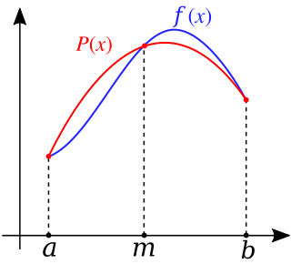
In calculus, Taylor's theorem gives an approximation of a -times differentiable function around a given point by a polynomial of degree , called the -th-order Taylor polynomial. For a smooth function, the Taylor polynomial is the truncation at the order of the Taylor series of the function. The first-order Taylor polynomial is the linear approximation of the function, and the second-order Taylor polynomial is often referred to as the quadratic approximation. There are several versions of Taylor's theorem, some giving explicit estimates of the approximation error of the function by its Taylor polynomial.

<span class="mw-page-title-main">Fourier transform</span> Mathematical transform that expresses a function of time as a function of frequency

In physics, engineering and mathematics, the Fourier transform (FT) is an integral transform that takes a function as input and outputs another function that describes the extent to which various frequencies are present in the original function. The output of the transform is a complex-valued function of frequency. The term Fourier transform refers to both this complex-valued function and the mathematical operation. When a distinction needs to be made the Fourier transform is sometimes called the frequency domain representation of the original function. The Fourier transform is analogous to decomposing the sound of a musical chord into the intensities of its constituent pitches.

In calculus, and more generally in mathematical analysis, integration by parts or partial integration is a process that finds the integral of a product of functions in terms of the integral of the product of their derivative and antiderivative. It is frequently used to transform the antiderivative of a product of functions into an antiderivative for which a solution can be more easily found. The rule can be thought of as an integral version of the product rule of differentiation; it is indeed derived using the product rule.

<span class="mw-page-title-main">Numerical integration</span> Methods of calculating definite integrals

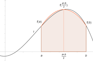
In analysis, numerical integration comprises a broad family of algorithms for calculating the numerical value of a definite integral. The term numerical quadrature is more or less a synonym for "numerical integration", especially as applied to one-dimensional integrals. Some authors refer to numerical integration over more than one dimension as cubature; others take "quadrature" to include higher-dimensional integration.

<span class="mw-page-title-main">Riemann sum</span> Approximation technique in integral calculus

In mathematics, a Riemann sum is a certain kind of approximation of an integral by a finite sum. It is named after nineteenth century German mathematician Bernhard Riemann. One very common application is in numerical integration, i.e., approximating the area of functions or lines on a graph, where it is also known as the rectangle rule. It can also be applied for approximating the length of curves and other approximations.

<span class="mw-page-title-main">Simpson's rule</span> Method for numerical integration

In numerical integration, Simpson's rules are several approximations for definite integrals, named after Thomas Simpson (1710–1761).

<span class="mw-page-title-main">Newton–Cotes formulas</span> Formulas for numerical integration

In numerical analysis, the Newton–Cotes formulas, also called the Newton–Cotes quadrature rules or simply Newton–Cotes rules, are a group of formulas for numerical integration based on evaluating the integrand at equally spaced points. They are named after Isaac Newton and Roger Cotes.

In vector calculus, Green's theorem relates a line integral around a simple closed curve C to a double integral over the plane region D bounded by C. It is the two-dimensional special case of Stokes' theorem.

<span class="mw-page-title-main">Differential operator</span> Typically linear operator defined in terms of differentiation of functions

In mathematics, a differential operator is an operator defined as a function of the differentiation operator. It is helpful, as a matter of notation first, to consider differentiation as an abstract operation that accepts a function and returns another function.

In mathematics, Laplace's method, named after Pierre-Simon Laplace, is a technique used to approximate integrals of the form

Particle filters, or sequential Monte Carlo methods, are a set of Monte Carlo algorithms used to find approximate solutions for filtering problems for nonlinear state-space systems, such as signal processing and Bayesian statistical inference. The filtering problem consists of estimating the internal states in dynamical systems when partial observations are made and random perturbations are present in the sensors as well as in the dynamical system. The objective is to compute the posterior distributions of the states of a Markov process, given the noisy and partial observations. The term "particle filters" was first coined in 1996 by Pierre Del Moral about mean-field interacting particle methods used in fluid mechanics since the beginning of the 1960s. The term "Sequential Monte Carlo" was coined by Jun S. Liu and Rong Chen in 1998.

In statistics and probability theory, a point process or point field is a collection of mathematical points randomly located on a mathematical space such as the real line or Euclidean space. Point processes can be used for spatial data analysis, which is of interest in such diverse disciplines as forestry, plant ecology, epidemiology, geography, seismology, materials science, astronomy, telecommunications, computational neuroscience, economics and others.

In calculus, the Leibniz integral rule for differentiation under the integral sign states that for an integral of the form

A product integral is any product-based counterpart of the usual sum-based integral of calculus. The first product integral was developed by the mathematician Vito Volterra in 1887 to solve systems of linear differential equations. Other examples of product integrals are the geometric integral, the bigeometric integral, and some other integrals of non-Newtonian calculus.

In mathematics, the spectral theory of ordinary differential equations is the part of spectral theory concerned with the determination of the spectrum and eigenfunction expansion associated with a linear ordinary differential equation. In his dissertation, Hermann Weyl generalized the classical Sturm–Liouville theory on a finite closed interval to second order differential operators with singularities at the endpoints of the interval, possibly semi-infinite or infinite. Unlike the classical case, the spectrum may no longer consist of just a countable set of eigenvalues, but may also contain a continuous part. In this case the eigenfunction expansion involves an integral over the continuous part with respect to a spectral measure, given by the Titchmarsh–Kodaira formula. The theory was put in its final simplified form for singular differential equations of even degree by Kodaira and others, using von Neumann's spectral theorem. It has had important applications in quantum mechanics, operator theory and harmonic analysis on semisimple Lie groups.

The uncertainty theory invented by Baoding Liu is a branch of mathematics based on normality, monotonicity, self-duality, countable subadditivity, and product measure axioms.

<span class="mw-page-title-main">Dirichlet kernel</span> Concept in mathematical analysis

In mathematical analysis, the Dirichlet kernel, named after the German mathematician Peter Gustav Lejeune Dirichlet, is the collection of periodic functions defined as

References