Slope

This article is about the mathematical term. For slope of a physical feature, see Grade (slope). For other uses, see Slope (disambiguation).

Slope: ${\displaystyle m={\frac {\Delta y}{\Delta x}}=\tan(\theta )}$

In mathematics, the slope or gradient of a line is a number that describes the direction of the line on a plane. ^[1] Often denoted by the letter m, slope is calculated as the ratio of the vertical change to the horizontal change ("rise over run") between two distinct points on the line, giving the same number for any choice of points.

The line may be physical – as set by a road surveyor, pictorial as in a diagram of a road or roof, or abstract. An application of the mathematical concept is found in the grade or gradient in geography and civil engineering.

The steepness, incline, or grade of a line is the absolute value of its slope: greater absolute value indicates a steeper line. The line trend is defined as follows:

• An "increasing" or "ascending" line goes up from left to right and has positive slope: ${\displaystyle m>0}$.
• A "decreasing" or "descending" line goes down from left to right and has negative slope: ${\displaystyle m<0}$.

Special directions are:

• A "(square) diagonal" line has unit slope: ${\displaystyle m=1}$
• A "horizontal" line (the graph of a constant function) has zero slope: ${\displaystyle m=0}$.
• A "vertical" line has undefined or infinite slope (see below).

If two points of a road have altitudes y₁ and y₂, the rise is the difference (y₂ − y₁) = Δy. Neglecting the Earth's curvature, if the two points have horizontal distance x₁ and x₂ from a fixed point, the run is (x₂ − x₁) = Δx. The slope between the two points is the difference ratio:

${\displaystyle m={\frac {\Delta y}{\Delta x}}={\frac {y_{2}-y_{1}}{x_{2}-x_{1}}}.}$

Through trigonometry, the slope m of a line is related to its angle of inclination θ by the tangent function

${\displaystyle m=\tan(\theta ).}$

Thus, a 45° rising line has slope m = +1, and a 45° falling line has slope m = −1.

Generalizing this, differential calculus defines the slope of a plane curve at a point as the slope of its tangent line at that point. When the curve is approximated by a series of points, the slope of the curve may be approximated by the slope of the secant line between two nearby points. When the curve is given as the graph of an algebraic expression, calculus gives formulas for the slope at each point. Slope is thus one of the central ideas of calculus and its applications to design.

Notation

There seems to be no clear answer as to why the letter m is used for slope, but it first appears in English in O'Brien (1844) ^[2] who introduced the equation of a line as "y = mx + b", and it can also be found in Todhunter (1888) ^[3] who wrote "y = mx + c". ^[4]

Definition

Slope illustrated for y = (3/2)x − 1. Click on to enlarge

Slope of a line in coordinates system, from f(x) = −12x + 2 to f(x) = 12x + 2

The slope of a line in the plane containing the x and y axes is generally represented by the letter m, ^[5] and is defined as the change in the y coordinate divided by the corresponding change in the x coordinate, between two distinct points on the line. This is described by the following equation:

${\displaystyle m={\frac {\Delta y}{\Delta x}}={\frac {{\text{vertical}}\,{\text{change}}}{{\text{horizontal}}\,{\text{change}}}}={\frac {\text{rise}}{\text{run}}}.}$

(The Greek letter delta , Δ, is commonly used in mathematics to mean "difference" or "change".)

Given two points ${\displaystyle (x_{1},y_{1})}$ and ${\displaystyle (x_{2},y_{2})}$, the change in ${\displaystyle x}$ from one to the other is ${\displaystyle x_{2}-x_{1}}$ (run), while the change in ${\displaystyle y}$ is ${\displaystyle y_{2}-y_{1}}$ (rise). Substituting both quantities into the above equation generates the formula:

${\displaystyle m={\frac {y_{2}-y_{1}}{x_{2}-x_{1}}}.}$

The formula fails for a vertical line, parallel to the ${\displaystyle y}$ axis (see Division by zero), where the slope can be taken as infinite, so the slope of a vertical line is considered undefined.

Examples

Suppose a line runs through two points: P = (1, 2) and Q = (13, 8). By dividing the difference in ${\displaystyle y}$-coordinates by the difference in ${\displaystyle x}$-coordinates, one can obtain the slope of the line:

${\displaystyle m={\frac {\Delta y}{\Delta x}}={\frac {y_{2}-y_{1}}{x_{2}-x_{1}}}={\frac {8-2}{13-1}}={\frac {6}{12}}={\frac {1}{2}}.}$

Since the slope is positive, the direction of the line is increasing. Since |m| < 1, the incline is not very steep (incline < 45°).

As another example, consider a line which runs through the points (4, 15) and (3, 21). Then, the slope of the line is

${\displaystyle m={\frac {21-15}{3-4}}={\frac {6}{-1}}=-6.}$

Since the slope is negative, the direction of the line is decreasing. Since |m| > 1, this decline is fairly steep (decline > 45°).

Algebra and geometry

Slopes of parallel and perpendicular lines

• If ${\displaystyle y}$ is a linear function of ${\displaystyle x}$, then the coefficient of ${\displaystyle x}$ is the slope of the line created by plotting the function. Therefore, if the equation of the line is given in the form

  ${\displaystyle y=mx+b}$

  then ${\displaystyle m}$ is the slope. This form of a line's equation is called the slope-intercept form, because ${\displaystyle b}$ can be interpreted as the y-intercept of the line, that is, the ${\displaystyle y}$-coordinate where the line intersects the ${\displaystyle y}$-axis.
• If the slope ${\displaystyle m}$ of a line and a point ${\displaystyle (x_{1},y_{1})}$ on the line are both known, then the equation of the line can be found using the point-slope formula:

  ${\displaystyle y-y_{1}=m(x-x_{1}).}$

• The slope of the line defined by the linear equation

  ${\displaystyle ax+by+c=0}$

  is

  ${\displaystyle -{\frac {a}{b}}}$.

• Two lines are parallel if and only if they are not the same line (coincident) and either their slopes are equal or they both are vertical and therefore both have undefined slopes.
• Two lines are perpendicular if the product of their slopes is −1 or one has a slope of 0 (a horizontal line) and the other has an undefined slope (a vertical line).
• The angle θ between −90° and 90° that a line makes with the x-axis is related to the slope m as follows:

  ${\displaystyle m=\tan(\theta )}$

  and

  ${\displaystyle \theta =\arctan(m)}$  (this is the inverse function of tangent; see inverse trigonometric functions).

Examples

For example, consider a line running through points (2,8) and (3,20). This line has a slope, m, of

${\displaystyle {\frac {(20-8)}{(3-2)}}=12.}$

One can then write the line's equation, in point-slope form:

${\displaystyle y-8=12(x-2)=12x-24.}$

or:

${\displaystyle y=12x-16.}$

The angle θ between −90° and 90° that this line makes with the x-axis is

${\displaystyle \theta =\arctan(12)\approx 85.2^{\circ }.}$

Consider the two lines: y = −3x + 1 and y = −3x − 2. Both lines have slope m = −3. They are not the same line. So they are parallel lines.

Consider the two lines y = −3x + 1 and y = ⁠x/3⁠ − 2. The slope of the first line is m₁ = −3. The slope of the second line is m₂ = ⁠1/3⁠. The product of these two slopes is −1. So these two lines are perpendicular.

Statistics

In statistics, the gradient of the least-squares regression best-fitting line for a given sample of data may be written as:

${\displaystyle m={\frac {rs_{y}}{s_{x}}}}$,

This quantity m is called as the regression slope for the line ${\displaystyle y=mx+c}$. The quantity ${\displaystyle r}$ is Pearson's correlation coefficient, ${\displaystyle s_{y}}$ is the standard deviation of the y-values and ${\displaystyle s_{x}}$ is the standard deviation of the x-values. This may also be written as a ratio of covariances: ^[6]

${\displaystyle m={\frac {\operatorname {cov} (Y,X)}{\operatorname {cov} (X,X)}}}$

Slope of a road or railway

Main articles: Grade (slope) and Grade separation

There are two common ways to describe the steepness of a road or railroad. One is by the angle between 0° and 90° (in degrees), and the other is by the slope in a percentage. See also steep grade railway and rack railway.

The formulae for converting a slope given as a percentage into an angle in degrees and vice versa are:

${\displaystyle {\text{angle}}=\arctan \left({\frac {\text{slope}}{100\%}}\right)}$ (this is the inverse function of tangent; see trigonometry)

and

${\displaystyle {\mbox{slope}}=100\%\times \tan({\mbox{angle}}),}$

where angle is in degrees and the trigonometric functions operate in degrees. For example, a slope of 100% or 1000‰ is an angle of 45°.

A third way is to give one unit of rise in say 10, 20, 50 or 100 horizontal units, e.g. 1:10. 1:20, 1:50 or 1:100 (or "1 in 10", "1 in 20", etc.) 1:10 is steeper than 1:20. For example, steepness of 20% means 1:5 or an incline with angle 11.3°.

Roads and railways have both longitudinal slopes and cross slopes.

• 
  Slope warning sign in the Netherlands
• 
  Slope warning sign in Poland
• 
  A 1371-meter distance of a railroad with a 20‰ slope. Czech Republic
• 
  Steam-age railway gradient post indicating a slope in both directions at Meols railway station, United Kingdom

Calculus

At each point, the derivative is the slope of a line that is tangent to the curve at that point. Note: the derivative at point A is positive where green and dash–dot, negative where red and dashed, and zero where black and solid.

The concept of a slope is central to differential calculus. For non-linear functions, the rate of change varies along the curve. The derivative of the function at a point is the slope of the line tangent to the curve at the point and is thus equal to the rate of change of the function at that point.

If we let Δx and Δy be the distances (along the x and y axes, respectively) between two points on a curve, then the slope given by the above definition,

${\displaystyle m={\frac {\Delta y}{\Delta x}}}$,

is the slope of a secant line to the curve. For a line, the secant between any two points is the line itself, but this is not the case for any other type of curve.

For example, the slope of the secant intersecting y = x² at (0,0) and (3,9) is 3. (The slope of the tangent at x = 3⁄2 is also 3 − a consequence of the mean value theorem.)

By moving the two points closer together so that Δy and Δx decrease, the secant line more closely approximates a tangent line to the curve, and as such the slope of the secant approaches that of the tangent. Using differential calculus, we can determine the limit, or the value that Δy/Δx approaches as Δy and Δx get closer to zero; it follows that this limit is the exact slope of the tangent. If y is dependent on x, then it is sufficient to take the limit where only Δx approaches zero. Therefore, the slope of the tangent is the limit of Δy/Δx as Δx approaches zero, or dy/dx. We call this limit the derivative.

${\displaystyle {\frac {\mathrm {d} y}{\mathrm {d} x}}=\lim _{\Delta x\to 0}{\frac {\Delta y}{\Delta x}}}$

The value of the derivative at a specific point on the function provides us with the slope of the tangent at that precise location. For example, let y = x². A point on this function is (−2,4). The derivative of this function is dy⁄dx = 2x. So the slope of the line tangent to y at (−2,4) is 2 ⋅ (−2) = −4. The equation of this tangent line is: y − 4 = (−4)(x − (−2)) or y = −4x − 4.

Difference of slopes

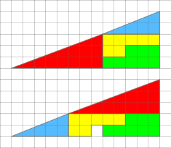
The illusion of a paradox of area is dispelled by comparing slopes where blue and red triangles meet.

An extension of the idea of angle follows from the difference of slopes. Consider the shear mapping

${\displaystyle (u,v)=(x,y){\begin{pmatrix}1&v\\0&1\end{pmatrix}}.}$

Then ${\displaystyle (1,0)}$ is mapped to ${\displaystyle (1,v)}$. The slope of ${\displaystyle (1,0)}$ is zero and the slope of ${\displaystyle (1,v)}$ is ${\displaystyle v}$. The shear mapping added a slope of ${\displaystyle v}$. For two points on ${\displaystyle \{(1,y):y\in \mathbb {R} \}}$ with slopes ${\displaystyle m}$ and ${\displaystyle n}$, the image

${\displaystyle (1,y){\begin{pmatrix}1&v\\0&1\end{pmatrix}}=(1,y+v)}$

has slope increased by ${\displaystyle v}$, but the difference ${\displaystyle n-m}$ of slopes is the same before and after the shear. This invariance of slope differences makes slope an angular invariant measure, on a par with circular angle (invariant under rotation) and hyperbolic angle, with invariance group of squeeze mappings. ^{[7] [8]}

Other uses

The concept of a slope or gradient is also used as a basis for developing other applications in mathematics:

• Gradient descent, a first-order iterative optimization algorithm for finding the minimum of a function
• Gradient theorem, theorem that a line integral through a gradient field can be evaluated by evaluating the original scalar field at the endpoints of the curve
• Gradient method, an algorithm to solve problems with search directions defined by the gradient of the function at the current point
• Conjugate gradient method, an algorithm for the numerical solution of particular systems of linear equations
• Nonlinear conjugate gradient method, generalizes the conjugate gradient method to nonlinear optimization
• Stochastic gradient descent, iterative method for optimizing a differentiable objective function

See also

• Euclidean distance
• Grade
• Inclined plane
• Linear function
• Line of greatest slope
• Mediant
• Slope definitions
• Theil–Sen estimator, a line with the median slope among a set of sample points

References

1. Clapham, C.; Nicholson, J. (2009). "Oxford Concise Dictionary of Mathematics, Gradient" (PDF). Addison-Wesley. p. 348. Archived from the original (PDF) on 29 October 2013. Retrieved 1 September 2013.
2. O'Brien, M. (1844), A Treatise on Plane Co-Ordinate Geometry or the Application of the Method of Co-Ordinates in the Solution of Problems in Plane Geometry, Cambridge, England: Deightons
3. Todhunter, I. (1888), Treatise on Plane Co-Ordinate Geometry as Applied to the Straight Line and Conic Sections, London: Macmillan
4. Weisstein, Eric W. "Slope". MathWorld--A Wolfram Web Resource. Archived from the original on 6 December 2016. Retrieved 30 October 2016.
5. An early example of this convention can be found in Salmon, George (1850). A Treatise on Conic Sections (2nd ed.). Dublin: Hodges and Smith. pp. 14–15.
6. Further Mathematics Units 3&4 VCE (Revised). Cambridge Senior Mathematics. 2016. ISBN   9781316616222 – via Physical Copy.
7. Bolt, Michael; Ferdinands, Timothy; Kavlie, Landon (2009). "The most general planar transformations that map parabolas into parabolas". Involve: A Journal of Mathematics. 2 (1): 79–88. doi: 10.2140/involve.2009.2.79 . ISSN   1944-4176. Archived from the original on 2020-06-12. Retrieved 2021-05-22.
8. Abstract Algebra/Shear and Slope at Wikibooks

External links

• "Slope of a Line (Coordinate Geometry)". Math Open Reference. 2009. Retrieved 30 October 2016. interactive