Pearson correlation coefficient

Not to be confused with Coefficient of determination.

Examples of scatter diagrams with different values of correlation coefficient (ρ)

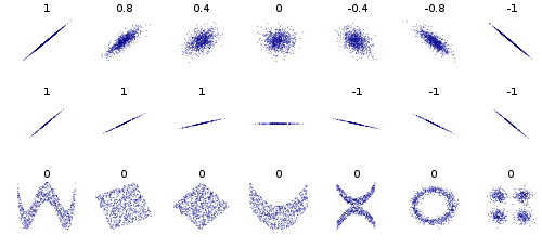
Several sets of (x, y) points, with the correlation coefficient of x and y for each set. The correlation reflects the strength and direction of a linear relationship (top row), but not the slope of that relationship (middle), nor many aspects of nonlinear relationships (bottom). N.B.: the figure in the center has a slope of 0 but in that case the correlation coefficient is undefined because the variance of Y is zero.

In statistics, the Pearson correlation coefficient (PCC) ^{[lower-alpha 1]} is a correlation coefficient that measures linear correlation between two sets of data. It is the ratio between the covariance of two variables and the product of their standard deviations; thus, it is essentially a normalized measurement of the covariance, such that the result always has a value between −1 and 1. As with covariance itself, the measure can only reflect a linear correlation of variables, and ignores many other types of relationships or correlations. As a simple example, one would expect the age and height of a sample of teenagers from a high school to have a Pearson correlation coefficient significantly greater than 0, but less than 1 (as 1 would represent an unrealistically perfect correlation).

Naming and history

It was developed by Karl Pearson from a related idea introduced by Francis Galton in the 1880s, and for which the mathematical formula was derived and published by Auguste Bravais in 1844. ^{[lower-alpha 2] [6] [7] [8] [9]} The naming of the coefficient is thus an example of Stigler's Law.

Definition

Pearson's correlation coefficient is the covariance of the two variables divided by the product of their standard deviations. The form of the definition involves a "product moment", that is, the mean (the first moment about the origin) of the product of the mean-adjusted random variables; hence the modifier product-moment in the name.^{[ verification needed ]}

For a population

Pearson's correlation coefficient, when applied to a population, is commonly represented by the Greek letter ρ (rho) and may be referred to as the population correlation coefficient or the population Pearson correlation coefficient. Given a pair of random variables ${\displaystyle (X,Y)}$ (for example, Height and Weight), the formula for ρ ^[10] is ^[11]

$${\displaystyle \rho _{X,Y}={\frac {\operatorname {cov} (X,Y)}{\sigma _{X}\sigma _{Y}}}}$$

where

• ${\displaystyle \operatorname {cov} }$ is the covariance
• ${\displaystyle \sigma _{X}}$ is the standard deviation of ${\displaystyle X}$
• ${\displaystyle \sigma _{Y}}$ is the standard deviation of ${\displaystyle Y}$.

The formula for ${\displaystyle \operatorname {cov} (X,Y)}$ can be expressed in terms of mean and expectation. Since ^[10]

${\displaystyle \operatorname {cov} (X,Y)=\operatorname {\mathbb {E} } [(X-\mu _{X})(Y-\mu _{Y})],}$

the formula for ${\displaystyle \rho }$ can also be written as

$${\displaystyle \rho _{X,Y}={\frac {\operatorname {\mathbb {E} } [(X-\mu _{X})(Y-\mu _{Y})]}{\sigma _{X}\sigma _{Y}}}}$$

where

• ${\displaystyle \sigma _{Y}}$ and ${\displaystyle \sigma _{X}}$ are defined as above
• ${\displaystyle \mu _{X}}$ is the mean of ${\displaystyle X}$
• ${\displaystyle \mu _{Y}}$ is the mean of ${\displaystyle Y}$
• ${\displaystyle \operatorname {\mathbb {E} } }$ is the expectation.

The formula for ${\displaystyle \rho }$ can be expressed in terms of uncentered moments. Since

${\displaystyle {\begin{aligned}\mu _{X}={}&\operatorname {\mathbb {E} } [\,X\,]\\\mu _{Y}={}&\operatorname {\mathbb {E} } [\,Y\,]\\\sigma _{X}^{2}={}&\operatorname {\mathbb {E} } \left[\,\left(X-\operatorname {\mathbb {E} } [X]\right)^{2}\,\right]=\operatorname {\mathbb {E} } \left[\,X^{2}\,\right]-\left(\operatorname {\mathbb {E} } [\,X\,]\right)^{2}\\\sigma _{Y}^{2}={}&\operatorname {\mathbb {E} } \left[\,\left(Y-\operatorname {\mathbb {E} } [Y]\right)^{2}\,\right]=\operatorname {\mathbb {E} } \left[\,Y^{2}\,\right]-\left(\,\operatorname {\mathbb {E} } [\,Y\,]\right)^{2}\\&\operatorname {\mathbb {E} } [\,\left(X-\mu _{X}\right)\left(Y-\mu _{Y}\right)\,]=\operatorname {\mathbb {E} } [\,\left(X-\operatorname {\mathbb {E} } [\,X\,]\right)\left(Y-\operatorname {\mathbb {E} } [\,Y\,]\right)\,]=\operatorname {\mathbb {E} } [\,X\,Y\,]-\operatorname {\mathbb {E} } [\,X\,]\operatorname {\mathbb {E} } [\,Y\,]\,,\end{aligned}}}$

the formula for ${\displaystyle \rho }$ can also be written as

$${\displaystyle \rho _{X,Y}={\frac {\operatorname {\mathbb {E} } [\,X\,Y\,]-\operatorname {\mathbb {E} } [\,X\,]\operatorname {\mathbb {E} } [\,Y\,]}{{\sqrt {\operatorname {\mathbb {E} } \left[\,X^{2}\,\right]-\left(\operatorname {\mathbb {E} } [\,X\,]\right)^{2}}}~{\sqrt {\operatorname {\mathbb {E} } \left[\,Y^{2}\,\right]-\left(\operatorname {\mathbb {E} } [\,Y\,]\right)^{2}}}}}.}$$

For a sample

Pearson's correlation coefficient, when applied to a sample, is commonly represented by ${\displaystyle r_{xy}}$ and may be referred to as the sample correlation coefficient or the sample Pearson correlation coefficient. We can obtain a formula for ${\displaystyle r_{xy}}$ by substituting estimates of the covariances and variances based on a sample into the formula above. Given paired data ${\displaystyle \left\{(x_{1},y_{1}),\ldots ,(x_{n},y_{n})\right\}}$ consisting of ${\displaystyle n}$ pairs, ${\displaystyle r_{xy}}$ is defined as

$${\displaystyle r_{xy}={\frac {\sum _{i=1}^{n}(x_{i}-{\bar {x}})(y_{i}-{\bar {y}})}{{\sqrt {\sum _{i=1}^{n}(x_{i}-{\bar {x}})^{2}}}{\sqrt {\sum _{i=1}^{n}(y_{i}-{\bar {y}})^{2}}}}}}$$

where

• ${\displaystyle n}$ is sample size
• ${\displaystyle x_{i},y_{i}}$ are the individual sample points indexed with i
• ${\textstyle {\bar {x}}={\frac {1}{n}}\sum _{i=1}^{n}x_{i}}$ (the sample mean); and analogously for ${\displaystyle {\bar {y}}}$.

Rearranging gives us this formula for ${\displaystyle r_{xy}}$:

${\displaystyle r_{xy}={\frac {n\sum x_{i}y_{i}-\sum x_{i}\sum y_{i}}{{\sqrt {n\sum x_{i}^{2}-\left(\sum x_{i}\right)^{2}}}~{\sqrt {n\sum y_{i}^{2}-\left(\sum y_{i}\right)^{2}}}}},}$

where ${\displaystyle n,x_{i},y_{i}}$ are defined as above.

This formula suggests a convenient single-pass algorithm for calculating sample correlations, though depending on the numbers involved, it can sometimes be numerically unstable.

Rearranging again gives us this ^[10] formula for ${\displaystyle r_{xy}}$:

${\displaystyle r_{xy}={\frac {\sum _{i}x_{i}y_{i}-n{\bar {x}}{\bar {y}}}{{\sqrt {\sum _{i}x_{i}^{2}-n{\bar {x}}^{2}}}~{\sqrt {\sum _{i}y_{i}^{2}-n{\bar {y}}^{2}}}}},}$

where ${\displaystyle n,x_{i},y_{i},{\bar {x}},{\bar {y}}}$ are defined as above.

An equivalent expression gives the formula for ${\displaystyle r_{xy}}$ as the mean of the products of the standard scores as follows:

${\displaystyle r_{xy}={\frac {1}{n-1}}\sum _{i=1}^{n}\left({\frac {x_{i}-{\bar {x}}}{s_{x}}}\right)\left({\frac {y_{i}-{\bar {y}}}{s_{y}}}\right)}$

where

• ${\displaystyle n,x_{i},y_{i},{\bar {x}},{\bar {y}}}$ are defined as above, and ${\displaystyle s_{x},s_{y}}$ are defined below
• ${\textstyle \left({\frac {x_{i}-{\bar {x}}}{s_{x}}}\right)}$ is the standard score (and analogously for the standard score of ${\displaystyle y}$).

Alternative formulae for ${\displaystyle r_{xy}}$ are also available. For example, one can use the following formula for ${\displaystyle r_{xy}}$:

${\displaystyle r_{xy}={\frac {\sum x_{i}y_{i}-n{\bar {x}}{\bar {y}}}{(n-1)s_{x}s_{y}}}}$

where

• ${\displaystyle n,x_{i},y_{i},{\bar {x}},{\bar {y}}}$ are defined as above and:
• ${\textstyle s_{x}={\sqrt {{\frac {1}{n-1}}\sum _{i=1}^{n}(x_{i}-{\bar {x}})^{2}}}}$ (the sample standard deviation); and analogously for ${\displaystyle s_{y}}$.

For jointly gaussian distributions

If ${\displaystyle (X,Y)}$ is jointly gaussian, with mean zero and variance ${\displaystyle \Sigma }$, then ${\displaystyle \Sigma ={\begin{bmatrix}\sigma _{X}^{2}&\rho _{X,Y}\sigma _{X}\sigma _{Y}\\\rho _{X,Y}\sigma _{X}\sigma _{Y}&\sigma _{Y}^{2}\\\end{bmatrix}}}$.

Practical issues

Under heavy noise conditions, extracting the correlation coefficient between two sets of stochastic variables is nontrivial, in particular where Canonical Correlation Analysis reports degraded correlation values due to the heavy noise contributions. A generalization of the approach is given elsewhere. ^[12]

In case of missing data, Garren derived the maximum likelihood estimator. ^[13]

Some distributions (e.g., stable distributions other than a normal distribution) do not have a defined variance.

Mathematical properties

The values of both the sample and population Pearson correlation coefficients are on or between −1 and 1. Correlations equal to +1 or −1 correspond to data points lying exactly on a line (in the case of the sample correlation), or to a bivariate distribution entirely supported on a line (in the case of the population correlation). The Pearson correlation coefficient is symmetric: corr(X,Y) = corr(Y,X).

A key mathematical property of the Pearson correlation coefficient is that it is invariant under separate changes in location and scale in the two variables. That is, we may transform X to a + bX and transform Y to c + dY, where a, b, c, and d are constants with b, d > 0, without changing the correlation coefficient. (This holds for both the population and sample Pearson correlation coefficients.) More general linear transformations do change the correlation: see § Decorrelation of n random variables for an application of this.

Interpretation

The correlation coefficient ranges from −1 to 1. An absolute value of exactly 1 implies that a linear equation describes the relationship between X and Y perfectly, with all data points lying on a line. The correlation sign is determined by the regression slope: a value of +1 implies that all data points lie on a line for which Y increases as X increases, whereas a value of -1 implies a line where Y increases while X decreases. ^[14] A value of 0 implies that there is no linear dependency between the variables. ^[15]

More generally, (X_i − X)(Y_i − Y) is positive if and only if X_i and Y_i lie on the same side of their respective means. Thus the correlation coefficient is positive if X_i and Y_i tend to be simultaneously greater than, or simultaneously less than, their respective means. The correlation coefficient is negative (anti-correlation) if X_i and Y_i tend to lie on opposite sides of their respective means. Moreover, the stronger either tendency is, the larger is the absolute value of the correlation coefficient.

Rodgers and Nicewander ^[16] cataloged thirteen ways of interpreting correlation or simple functions of it:

• Function of raw scores and means
• Standardized covariance
• Standardized slope of the regression line
• Geometric mean of the two regression slopes
• Square root of the ratio of two variances
• Mean cross-product of standardized variables
• Function of the angle between two standardized regression lines
• Function of the angle between two variable vectors
• Rescaled variance of the difference between standardized scores
• Estimated from the balloon rule
• Related to the bivariate ellipses of isoconcentration
• Function of test statistics from designed experiments
• Ratio of two means

Geometric interpretation

Regression lines for y = g_X(x) [red] and x = g_Y(y) [blue]

For uncentered data, there is a relation between the correlation coefficient and the angle φ between the two regression lines, y = g_X(x) and x = g_Y(y), obtained by regressing y on x and x on y respectively. (Here, φ is measured counterclockwise within the first quadrant formed around the lines' intersection point if r > 0, or counterclockwise from the fourth to the second quadrant if r < 0.) One can show ^[17] that if the standard deviations are equal, then r = sec φ − tan φ, where sec and tan are trigonometric functions.

For centered data (i.e., data which have been shifted by the sample means of their respective variables so as to have an average of zero for each variable), the correlation coefficient can also be viewed as the cosine of the angle θ between the two observed vectors in N-dimensional space (for N observations of each variable). ^[18]

Both the uncentered (non-Pearson-compliant) and centered correlation coefficients can be determined for a dataset. As an example, suppose five countries are found to have gross national products of 1, 2, 3, 5, and 8 billion dollars, respectively. Suppose these same five countries (in the same order) are found to have 11%, 12%, 13%, 15%, and 18% poverty. Then let x and y be ordered 5-element vectors containing the above data: x = (1, 2, 3, 5, 8) and y = (0.11, 0.12, 0.13, 0.15, 0.18).

By the usual procedure for finding the angle θ between two vectors (see dot product), the uncentered correlation coefficient is

${\displaystyle \cos \theta ={\frac {\mathbf {x} \cdot \mathbf {y} }{\left\|\mathbf {x} \right\|\left\|\mathbf {y} \right\|}}={\frac {2.93}{{\sqrt {103}}{\sqrt {0.0983}}}}=0.920814711.}$

This uncentered correlation coefficient is identical with the cosine similarity. The above data were deliberately chosen to be perfectly correlated: y = 0.10 + 0.01 x. The Pearson correlation coefficient must therefore be exactly one. Centering the data (shifting x by ℰ(x) = 3.8 and y by ℰ(y) = 0.138) yields x = (−2.8, −1.8, −0.8, 1.2, 4.2) and y = (−0.028, −0.018, −0.008, 0.012, 0.042), from which

${\displaystyle \cos \theta ={\frac {\mathbf {x} \cdot \mathbf {y} }{\left\|\mathbf {x} \right\|\left\|\mathbf {y} \right\|}}={\frac {0.308}{{\sqrt {30.8}}{\sqrt {0.00308}}}}=1=\rho _{xy},}$

as expected.

Interpretation of the size of a correlation

This figure gives a sense of how the usefulness of a Pearson correlation for predicting values varies with its magnitude. Given jointly normal X, Y with correlation ρ, ${\displaystyle 1-{\sqrt {1-\rho ^{2}}}}$ (plotted here as a function of ρ) is the factor by which a given prediction interval for Y may be reduced given the corresponding value of X. For example, if ρ = 0.5, then the 95% prediction interval of Y|X will be about 13% smaller than the 95% prediction interval of Y.

Several authors have offered guidelines for the interpretation of a correlation coefficient. ^{[19] [20]} However, all such criteria are in some ways arbitrary. ^[20] The interpretation of a correlation coefficient depends on the context and purposes. A correlation of 0.8 may be very low if one is verifying a physical law using high-quality instruments, but may be regarded as very high in the social sciences, where there may be a greater contribution from complicating factors.

Inference

Statistical inference based on Pearson's correlation coefficient often focuses on one of the following two aims:

• One aim is to test the null hypothesis that the true correlation coefficient ρ is equal to 0, based on the value of the sample correlation coefficient r.
• The other aim is to derive a confidence interval that, on repeated sampling, has a given probability of containing ρ.

Methods of achieving one or both of these aims are discussed below.

Using a permutation test

Permutation tests provide a direct approach to performing hypothesis tests and constructing confidence intervals. A permutation test for Pearson's correlation coefficient involves the following two steps:

1. Using the original paired data (x_i, y_i), randomly redefine the pairs to create a new data set (x_i, y_i′), where the i′ are a permutation of the set {1,...,n}. The permutation i′ is selected randomly, with equal probabilities placed on all n! possible permutations. This is equivalent to drawing the i′ randomly without replacement from the set {1, ..., n}. In bootstrapping, a closely related approach, the i and the i′ are equal and drawn with replacement from {1, ..., n};
2. Construct a correlation coefficient r from the randomized data.

To perform the permutation test, repeat steps (1) and (2) a large number of times. The p-value for the permutation test is the proportion of the r values generated in step (2) that are larger than the Pearson correlation coefficient that was calculated from the original data. Here "larger" can mean either that the value is larger in magnitude, or larger in signed value, depending on whether a two-sided or one-sided test is desired.

Using a bootstrap

The bootstrap can be used to construct confidence intervals for Pearson's correlation coefficient. In the "non-parametric" bootstrap, n pairs (x_i, y_i) are resampled "with replacement" from the observed set of n pairs, and the correlation coefficient r is calculated based on the resampled data. This process is repeated a large number of times, and the empirical distribution of the resampled r values are used to approximate the sampling distribution of the statistic. A 95% confidence interval for ρ can be defined as the interval spanning from the 2.5th to the 97.5th percentile of the resampled r values.

Standard error

If ${\displaystyle x}$ and ${\displaystyle y}$ are random variables, a standard error associated to the correlation in the null case is

${\displaystyle \sigma _{r}={\sqrt {\frac {1-r^{2}}{n-2}}}}$

where ${\displaystyle r}$ is the correlation (assumed r≈0) and ${\displaystyle n}$ the sample size. ^{[21] [22]}

Testing using Student's t-distribution

Critical values of Pearson's correlation coefficient that must be exceeded to be considered significantly nonzero at the 0.05 level

For pairs from an uncorrelated bivariate normal distribution, the sampling distribution of the studentized Pearson's correlation coefficient follows Student's t-distribution with degrees of freedom n − 2. Specifically, if the underlying variables have a bivariate normal distribution, the variable

${\displaystyle t={\frac {r}{\sigma _{r}}}=r{\sqrt {\frac {n-2}{1-r^{2}}}}}$

has a student's t-distribution in the null case (zero correlation). ^[23] This holds approximately in case of non-normal observed values if sample sizes are large enough. ^[24] For determining the critical values for r the inverse function is needed:

${\displaystyle r={\frac {t}{\sqrt {n-2+t^{2}}}}.}$

Alternatively, large sample, asymptotic approaches can be used.

Another early paper ^[25] provides graphs and tables for general values of ρ, for small sample sizes, and discusses computational approaches.

In the case where the underlying variables are not normal, the sampling distribution of Pearson's correlation coefficient follows a Student's t-distribution, but the degrees of freedom are reduced. ^[26]

Using the exact distribution

For data that follow a bivariate normal distribution, the exact density function f(r) for the sample correlation coefficient r of a normal bivariate is ^{[27] [28] [29]}

${\displaystyle f(r)={\frac {(n-2)\,\mathrm {\Gamma } (n-1)\left(1-\rho ^{2}\right)^{\frac {n-1}{2}}\left(1-r^{2}\right)^{\frac {n-4}{2}}}{{\sqrt {2\pi }}\,\operatorname {\Gamma } {\mathord {\left(n-{\tfrac {1}{2}}\right)}}(1-\rho r)^{n-{\frac {3}{2}}}}}{}_{2}\mathrm {F} _{1}{\mathord {\left({\tfrac {1}{2}},{\tfrac {1}{2}};{\tfrac {1}{2}}(2n-1);{\tfrac {1}{2}}(\rho r+1)\right)}}}$

where ${\displaystyle \Gamma }$ is the gamma function and ${\displaystyle {}_{2}\mathrm {F} _{1}(a,b;c;z)}$ is the Gaussian hypergeometric function.

In the special case when ${\displaystyle \rho =0}$ (zero population correlation), the exact density function f(r) can be written as

${\displaystyle f(r)={\frac {\left({\frac {1}{1-r^{2}}}\right)^{-{\frac {n-1}{2}}}}{{\sqrt {n-2}}\,\operatorname {\mathrm {B} } {\mathord {\left({\tfrac {1}{2}},{\tfrac {n-2}{2}}\right)}}}},}$

where ${\displaystyle \mathrm {B} }$ is the beta function, which is one way of writing the density of a Student's t-distribution for a studentized sample correlation coefficient, as above.

Using the exact confidence distribution

Confidence intervals and tests can be calculated from a confidence distribution. An exact confidence density for ρ is ^[30]

$${\displaystyle \pi (\rho \mid r)={\frac {\nu (\nu -1)\Gamma (\nu -1)}{{\sqrt {2\pi }}\Gamma \left(\nu +{\frac {1}{2}}\right)}}\left(1-r^{2}\right)^{\frac {\nu -1}{2}}\cdot \left(1-\rho ^{2}\right)^{\frac {\nu -2}{2}}\cdot \left(1-r\rho \right)^{\frac {1-2\nu }{2}}\operatorname {F} \left({\tfrac {3}{2}},-{\tfrac {1}{2}};\nu +{\tfrac {1}{2}};{\tfrac {1+r\rho }{2}}\right)}$$

where ${\displaystyle \operatorname {F} }$ is the Gaussian hypergeometric function and ${\displaystyle \nu =n-1>1}$.

Using the Fisher transformation

Main article: Fisher transformation

In practice, confidence intervals and hypothesis tests relating to ρ are usually carried out using the Fisher transformation, ${\displaystyle F}$:

${\displaystyle F(r)\equiv {\tfrac {1}{2}}\,\ln \left({\frac {1+r}{1-r}}\right)=\operatorname {artanh} (r)}$

F(r) approximately follows a normal distribution with

${\displaystyle {\text{mean}}=F(\rho )=\operatorname {artanh} (\rho )}$    and standard error ${\displaystyle ={\text{SE}}={\frac {1}{\sqrt {n-3}}},}$

where n is the sample size. The approximation error is lowest for a large sample size ${\displaystyle n}$ and small ${\displaystyle r}$ and ${\displaystyle \rho _{0}}$ and increases otherwise.

Using the approximation, a z-score is

${\displaystyle z={\frac {x-{\text{mean}}}{\text{SE}}}=[F(r)-F(\rho _{0})]{\sqrt {n-3}}}$

under the null hypothesis that ${\displaystyle \rho =\rho _{0}}$, given the assumption that the sample pairs are independent and identically distributed and follow a bivariate normal distribution. Thus an approximate p-value can be obtained from a normal probability table. For example, if z = 2.2 is observed and a two-sided p-value is desired to test the null hypothesis that ${\displaystyle \rho =0}$, the p-value is 2 Φ(−2.2) = 0.028, where Φ is the standard normal cumulative distribution function.

To obtain a confidence interval for ρ, we first compute a confidence interval for F(${\displaystyle \rho }$):

${\displaystyle 100(1-\alpha )\%{\text{CI}}:\operatorname {artanh} (\rho )\in [\operatorname {artanh} (r)\pm z_{\alpha /2}{\text{SE}}]}$

The inverse Fisher transformation brings the interval back to the correlation scale.

${\displaystyle 100(1-\alpha )\%{\text{CI}}:\rho \in [\tanh(\operatorname {artanh} (r)-z_{\alpha /2}{\text{SE}}),\tanh(\operatorname {artanh} (r)+z_{\alpha /2}{\text{SE}})]}$

For example, suppose we observe r = 0.7 with a sample size of n=50, and we wish to obtain a 95% confidence interval for ρ. The transformed value is ${\textstyle \operatorname {arctanh} \left(r\right)=0.8673}$, so the confidence interval on the transformed scale is ${\displaystyle 0.8673\pm {\frac {1.96}{\sqrt {47}}}}$, or (0.5814, 1.1532). Converting back to the correlation scale yields (0.5237, 0.8188).

In least squares regression analysis

For more general, non-linear dependency, see Coefficient of determination § In a multiple linear model.

The square of the sample correlation coefficient is typically denoted r² and is a special case of the coefficient of determination. In this case, it estimates the fraction of the variance in Y that is explained by X in a simple linear regression. So if we have the observed dataset ${\displaystyle Y_{1},\dots ,Y_{n}}$ and the fitted dataset ${\displaystyle {\hat {Y}}_{1},\dots ,{\hat {Y}}_{n}}$ then as a starting point the total variation in the Y_i around their average value can be decomposed as follows

${\displaystyle \sum _{i}(Y_{i}-{\bar {Y}})^{2}=\sum _{i}(Y_{i}-{\hat {Y}}_{i})^{2}+\sum _{i}({\hat {Y}}_{i}-{\bar {Y}})^{2},}$

where the ${\displaystyle {\hat {Y}}_{i}}$ are the fitted values from the regression analysis. This can be rearranged to give

${\displaystyle 1={\frac {\sum _{i}(Y_{i}-{\hat {Y}}_{i})^{2}}{\sum _{i}(Y_{i}-{\bar {Y}})^{2}}}+{\frac {\sum _{i}({\hat {Y}}_{i}-{\bar {Y}})^{2}}{\sum _{i}(Y_{i}-{\bar {Y}})^{2}}}.}$

The two summands above are the fraction of variance in Y that is explained by X (right) and that is unexplained by X (left).

Next, we apply a property of least square regression models, that the sample covariance between ${\displaystyle {\hat {Y}}_{i}}$ and ${\displaystyle Y_{i}-{\hat {Y}}_{i}}$ is zero. Thus, the sample correlation coefficient between the observed and fitted response values in the regression can be written (calculation is under expectation, assumes Gaussian statistics)

${\displaystyle {\begin{aligned}r(Y,{\hat {Y}})&={\frac {\sum _{i}(Y_{i}-{\bar {Y}})({\hat {Y}}_{i}-{\bar {Y}})}{\sqrt {\sum _{i}(Y_{i}-{\bar {Y}})^{2}\cdot \sum _{i}({\hat {Y}}_{i}-{\bar {Y}})^{2}}}}\\[6pt]&={\frac {\sum _{i}(Y_{i}-{\hat {Y}}_{i}+{\hat {Y}}_{i}-{\bar {Y}})({\hat {Y}}_{i}-{\bar {Y}})}{\sqrt {\sum _{i}(Y_{i}-{\bar {Y}})^{2}\cdot \sum _{i}({\hat {Y}}_{i}-{\bar {Y}})^{2}}}}\\[6pt]&={\frac {\sum _{i}[(Y_{i}-{\hat {Y}}_{i})({\hat {Y}}_{i}-{\bar {Y}})+({\hat {Y}}_{i}-{\bar {Y}})^{2}]}{\sqrt {\sum _{i}(Y_{i}-{\bar {Y}})^{2}\cdot \sum _{i}({\hat {Y}}_{i}-{\bar {Y}})^{2}}}}\\[6pt]&={\frac {\sum _{i}({\hat {Y}}_{i}-{\bar {Y}})^{2}}{\sqrt {\sum _{i}(Y_{i}-{\bar {Y}})^{2}\cdot \sum _{i}({\hat {Y}}_{i}-{\bar {Y}})^{2}}}}\\[6pt]&={\sqrt {\frac {\sum _{i}({\hat {Y}}_{i}-{\bar {Y}})^{2}}{\sum _{i}(Y_{i}-{\bar {Y}})^{2}}}}.\end{aligned}}}$

Thus

${\displaystyle r(Y,{\hat {Y}})^{2}={\frac {\sum _{i}({\hat {Y}}_{i}-{\bar {Y}})^{2}}{\sum _{i}(Y_{i}-{\bar {Y}})^{2}}}}$

where ${\displaystyle r(Y,{\hat {Y}})^{2}}$ is the proportion of variance in Y explained by a linear function of X.

In the derivation above, the fact that

${\displaystyle \sum _{i}(Y_{i}-{\hat {Y}}_{i})({\hat {Y}}_{i}-{\bar {Y}})=0}$

can be proved by noticing that the partial derivatives of the residual sum of squares (RSS) over β₀ and β₁ are equal to 0 in the least squares model, where

${\displaystyle {\text{RSS}}=\sum _{i}(Y_{i}-{\hat {Y}}_{i})^{2}}$.

In the end, the equation can be written as

${\displaystyle r(Y,{\hat {Y}})^{2}={\frac {{\text{SS}}_{\text{reg}}}{{\text{SS}}_{\text{tot}}}}}$

where

• ${\displaystyle {\text{SS}}_{\text{reg}}=\sum _{i}({\hat {Y}}_{i}-{\bar {Y}})^{2}}$
• ${\displaystyle {\text{SS}}_{\text{tot}}=\sum _{i}(Y_{i}-{\bar {Y}})^{2}}$.

The symbol ${\displaystyle {\text{SS}}_{\text{reg}}}$ is called the regression sum of squares, also called the explained sum of squares, and ${\displaystyle {\text{SS}}_{\text{tot}}}$ is the total sum of squares (proportional to the variance of the data).

Sensitivity to the data distribution

Further information: Correlation and dependence § Sensitivity to the data distribution

Existence

The population Pearson correlation coefficient is defined in terms of moments, and therefore exists for any bivariate probability distribution for which the population covariance is defined and the marginal population variances are defined and are non-zero. Some probability distributions, such as the Cauchy distribution, have undefined variance and hence ρ is not defined if X or Y follows such a distribution. In some practical applications, such as those involving data suspected to follow a heavy-tailed distribution, this is an important consideration. However, the existence of the correlation coefficient is usually not a concern; for instance, if the range of the distribution is bounded, ρ is always defined.

Sample size

• If the sample size is moderate or large and the population is normal, then, in the case of the bivariate normal distribution, the sample correlation coefficient is the maximum likelihood estimate of the population correlation coefficient, and is asymptotically unbiased and efficient, which roughly means that it is impossible to construct a more accurate estimate than the sample correlation coefficient.
• If the sample size is large and the population is not normal, then the sample correlation coefficient remains approximately unbiased, but may not be efficient.
• If the sample size is large, then the sample correlation coefficient is a consistent estimator of the population correlation coefficient as long as the sample means, variances, and covariance are consistent (which is guaranteed when the law of large numbers can be applied).
• If the sample size is small, then the sample correlation coefficient r is not an unbiased estimate of ρ. ^[10] The adjusted correlation coefficient must be used instead: see elsewhere in this article for the definition.
• Correlations can be different for imbalanced dichotomous data when there is variance error in sample. ^[31]

Robustness

Like many commonly used statistics, the sample statistic r is not robust, ^[32] so its value can be misleading if outliers are present. ^{[33] [34]} Specifically, the PMCC is neither distributionally robust, ^[35] nor outlier resistant ^[32] (see Robust statistics § Definition ). Inspection of the scatterplot between X and Y will typically reveal a situation where lack of robustness might be an issue, and in such cases it may be advisable to use a robust measure of association. Note however that while most robust estimators of association measure statistical dependence in some way, they are generally not interpretable on the same scale as the Pearson correlation coefficient.

Statistical inference for Pearson's correlation coefficient is sensitive to the data distribution. Exact tests, and asymptotic tests based on the Fisher transformation can be applied if the data are approximately normally distributed, but may be misleading otherwise. In some situations, the bootstrap can be applied to construct confidence intervals, and permutation tests can be applied to carry out hypothesis tests. These non-parametric approaches may give more meaningful results in some situations where bivariate normality does not hold. However the standard versions of these approaches rely on exchangeability of the data, meaning that there is no ordering or grouping of the data pairs being analyzed that might affect the behavior of the correlation estimate.

A stratified analysis is one way to either accommodate a lack of bivariate normality, or to isolate the correlation resulting from one factor while controlling for another. If W represents cluster membership or another factor that it is desirable to control, we can stratify the data based on the value of W, then calculate a correlation coefficient within each stratum. The stratum-level estimates can then be combined to estimate the overall correlation while controlling for W. ^[36]

Variants

See also: Correlation and dependence § Other measures of dependence among random variables

Variations of the correlation coefficient can be calculated for different purposes. Here are some examples.

Adjusted correlation coefficient

The sample correlation coefficient r is not an unbiased estimate of ρ. For data that follows a bivariate normal distribution, the expectation E[r] for the sample correlation coefficient r of a normal bivariate is ^[37]

${\displaystyle \operatorname {\mathbb {E} } \left[r\right]=\rho -{\frac {\rho \left(1-\rho ^{2}\right)}{2n}}+\cdots ,\quad }$ therefore r is a biased estimator of ${\displaystyle \rho .}$

The unique minimum variance unbiased estimator r_adj is given by ^[38]

${\displaystyle r_{\text{adj}}=r\,\mathbf {_{2}F_{1}} \left({\frac {1}{2}},{\frac {1}{2}};{\frac {n-1}{2}};1-r^{2}\right),}$

(1)

where:

• ${\displaystyle r,n}$ are defined as above,
• ${\displaystyle \mathbf {_{2}F_{1}} (a,b;c;z)}$ is the Gaussian hypergeometric function.

An approximately unbiased estimator r_adj can be obtained^{[ citation needed ]} by truncating E[r] and solving this truncated equation:

${\displaystyle r=\operatorname {\mathbb {E} } [r]\approx r_{\text{adj}}-{\frac {r_{\text{adj}}\left(1-r_{\text{adj}}^{2}\right)}{2n}}.}$

(2)

An approximate solution^{[ citation needed ]} to equation ( 2 ) is

${\displaystyle r_{\text{adj}}\approx r\left[1+{\frac {1-r^{2}}{2n}}\right],}$

(3)

where in ( 3 )

• ${\displaystyle r,n}$ are defined as above,
• r_adj is a suboptimal estimator,^{[ citation needed ][ clarification needed ]}
• r_adj can also be obtained by maximizing log(f(r)),
• r_adj has minimum variance for large values of n,
• r_adj has a bias of order 1⁄(n − 1).

Another proposed ^[10] adjusted correlation coefficient is^{[ citation needed ]}

${\displaystyle r_{\text{adj}}={\sqrt {1-{\frac {(1-r^{2})(n-1)}{(n-2)}}}}.}$

r_adj ≈ r for large values of n.

Weighted correlation coefficient

Suppose observations to be correlated have differing degrees of importance that can be expressed with a weight vector w. To calculate the correlation between vectors x and y with the weight vector w (all of length n), ^{[39] [40]}

• Weighted mean:
  $${\displaystyle \operatorname {m} (x;w)={\frac {\sum _{i}w_{i}x_{i}}{\sum _{i}w_{i}}}.}$$
• Weighted covariance
  $${\displaystyle \operatorname {cov} (x,y;w)={\frac {\sum _{i}w_{i}\cdot (x_{i}-\operatorname {m} (x;w))(y_{i}-\operatorname {m} (y;w))}{\sum _{i}w_{i}}}.}$$
• Weighted correlation
  $${\displaystyle \operatorname {corr} (x,y;w)={\frac {\operatorname {cov} (x,y;w)}{\sqrt {\operatorname {cov} (x,x;w)\operatorname {cov} (y,y;w)}}}.}$$

Reflective correlation coefficient

The reflective correlation is a variant of Pearson's correlation in which the data are not centered around their mean values.^{[ citation needed ]} The population reflective correlation is

${\displaystyle \operatorname {corr} _{r}(X,Y)={\frac {\operatorname {\mathbb {E} } [\,X\,Y\,]}{\sqrt {\operatorname {\mathbb {E} } [\,X^{2}\,]\cdot \operatorname {\mathbb {E} } [\,Y^{2}\,]}}}.}$

The reflective correlation is symmetric, but it is not invariant under translation:

${\displaystyle \operatorname {corr} _{r}(X,Y)=\operatorname {corr} _{r}(Y,X)=\operatorname {corr} _{r}(X,bY)\neq \operatorname {corr} _{r}(X,a+bY),\quad a\neq 0,b>0.}$

The sample reflective correlation is equivalent to cosine similarity:

${\displaystyle rr_{xy}={\frac {\sum x_{i}y_{i}}{\sqrt {(\sum x_{i}^{2})(\sum y_{i}^{2})}}}.}$

The weighted version of the sample reflective correlation is

${\displaystyle rr_{xy,w}={\frac {\sum w_{i}x_{i}y_{i}}{\sqrt {(\sum w_{i}x_{i}^{2})(\sum w_{i}y_{i}^{2})}}}.}$

Scaled correlation coefficient

Main article: Scaled correlation

Scaled correlation is a variant of Pearson's correlation in which the range of the data is restricted intentionally and in a controlled manner to reveal correlations between fast components in time series. ^[41] Scaled correlation is defined as average correlation across short segments of data.

Let ${\displaystyle K}$ be the number of segments that can fit into the total length of the signal ${\displaystyle T}$ for a given scale ${\displaystyle s}$:

${\displaystyle K=\operatorname {round} \left({\frac {T}{s}}\right).}$

The scaled correlation across the entire signals ${\displaystyle {\bar {r}}_{s}}$ is then computed as

${\displaystyle {\bar {r}}_{s}={\frac {1}{K}}\sum \limits _{k=1}^{K}r_{k},}$

where ${\displaystyle r_{k}}$ is Pearson's coefficient of correlation for segment ${\displaystyle k}$.

By choosing the parameter ${\displaystyle s}$, the range of values is reduced and the correlations on long time scale are filtered out, only the correlations on short time scales being revealed. Thus, the contributions of slow components are removed and those of fast components are retained.

Pearson's distance

A distance metric for two variables X and Y known as Pearson's distance can be defined from their correlation coefficient as ^[42]

${\displaystyle d_{X,Y}=1-\rho _{X,Y}.}$

Considering that the Pearson correlation coefficient falls between [−1, +1], the Pearson distance lies in [0, 2]. The Pearson distance has been used in cluster analysis and data detection for communications and storage with unknown gain and offset. ^[43]

The Pearson "distance" defined this way assigns distance greater than 1 to negative correlations. In reality, both strong positive correlation and negative correlations are meaningful, so care must be taken when Pearson "distance" is used for nearest neighbor algorithm as such algorithm will only include neighbors with positive correlation and exclude neighbors with negative correlation. Alternatively, an absolute valued distance, ${\displaystyle d_{X,Y}=1-|\rho _{X,Y}|}$, can be applied, which will take both positive and negative correlations into consideration. The information on positive and negative association can be extracted separately, later.

Circular correlation coefficient

Further information: Circular statistics

For variables X = {x₁,...,x_n} and Y = {y₁,...,y_n} that are defined on the unit circle [0, 2π), it is possible to define a circular analog of Pearson's coefficient. ^[44] This is done by transforming data points in X and Y with a sine function such that the correlation coefficient is given as:

${\displaystyle r_{\text{circular}}={\frac {\sum _{i=1}^{n}\sin(x_{i}-{\bar {x}})\sin(y_{i}-{\bar {y}})}{{\sqrt {\sum _{i=1}^{n}\sin(x_{i}-{\bar {x}})^{2}}}{\sqrt {\sum _{i=1}^{n}\sin(y_{i}-{\bar {y}})^{2}}}}}}$

where ${\displaystyle {\bar {x}}}$ and ${\displaystyle {\bar {y}}}$ are the circular means of X and Y. This measure can be useful in fields like meteorology where the angular direction of data is important.

Partial correlation

Main article: Partial correlation

If a population or data-set is characterized by more than two variables, a partial correlation coefficient measures the strength of dependence between a pair of variables that is not accounted for by the way in which they both change in response to variations in a selected subset of the other variables.

Decorrelation of n random variables

Main article: Decorrelation

It is always possible to remove the correlations between all pairs of an arbitrary number of random variables by using a data transformation, even if the relationship between the variables is nonlinear. A presentation of this result for population distributions is given by Cox & Hinkley. ^[45]

A corresponding result exists for reducing the sample correlations to zero. Suppose a vector of n random variables is observed m times. Let X be a matrix where ${\displaystyle X_{i,j}}$ is the jth variable of observation i. Let ${\displaystyle Z_{m,m}}$ be an m by m square matrix with every element 1. Then D is the data transformed so every random variable has zero mean, and T is the data transformed so all variables have zero mean and zero correlation with all other variables – the sample correlation matrix of T will be the identity matrix. This has to be further divided by the standard deviation to get unit variance. The transformed variables will be uncorrelated, even though they may not be independent.

${\displaystyle D=X-{\frac {1}{m}}Z_{m,m}X}$

${\displaystyle T=D(D^{\mathsf {T}}D)^{-{\frac {1}{2}}},}$

where an exponent of −+1⁄2 represents the matrix square root of the inverse of a matrix. The correlation matrix of T will be the identity matrix. If a new data observation x is a row vector of n elements, then the same transform can be applied to x to get the transformed vectors d and t:

${\displaystyle d=x-{\frac {1}{m}}Z_{1,m}X,}$

${\displaystyle t=d(D^{\mathsf {T}}D)^{-{\frac {1}{2}}}.}$

This decorrelation is related to principal components analysis for multivariate data.

Software implementations

• R's statistics base-package implements the correlation coefficient with cor(x, y), or (with the P value also) with cor.test(x, y).
• The SciPy Python library via pearsonr(x, y).
• The Pandas Python library implements Pearson correlation coefficient calculation as the default option for the method pandas.DataFrame.corr
• Wolfram Mathematica via the Correlation function, or (with the P value) with CorrelationTest.
• The Boost C++ library via the correlation_coefficient function.
• Excel has an in-built correl(array1, array2) function for calculating the pearson's correlation coefficient.

See also

• Mathematics portal

• Anscombe's quartet
• Association (statistics)
• Coefficient of colligation
  • Yule's Q
  • Yule's Y
• Coefficient of multiple correlation
• Concordance correlation coefficient
• Correlation and dependence
• Correlation ratio
• Disattenuation
• Distance correlation
• Maximal information coefficient
• Multiple correlation
• Normally distributed and uncorrelated does not imply independent
• Odds ratio
• Partial correlation
• Polychoric correlation
• Quadrant count ratio
• RV coefficient
• Spearman's rank correlation coefficient

Footnotes

1. Also known as Pearson's r, the Pearson product-moment correlation coefficient (PPMCC), the bivariate correlation, ^[1] or simply the unqualified correlation coefficient ^[2]
2. As early as 1877, Galton was using the term "reversion" and the symbol "r" for what would become "regression". ^{[3] [4] [5]}

References

1. "SPSS Tutorials: Pearson Correlation".
2. "Correlation Coefficient: Simple Definition, Formula, Easy Steps". Statistics How To.
3. Galton, F. (5–19 April 1877). "Typical laws of heredity". Nature. 15 (388, 389, 390): 492–495, 512–514, 532–533. Bibcode:1877Natur..15..492.. doi: 10.1038/015492a0 . S2CID   4136393. In the "Appendix" on page 532, Galton uses the term "reversion" and the symbol r.
4. Galton, F. (24 September 1885). "The British Association: Section II, Anthropology: Opening address by Francis Galton, F.R.S., etc., President of the Anthropological Institute, President of the Section". Nature. 32 (830): 507–510.
5. Galton, F. (1886). "Regression towards mediocrity in hereditary stature". Journal of the Anthropological Institute of Great Britain and Ireland. 15: 246–263. doi:10.2307/2841583. JSTOR   2841583.
6. Pearson, Karl (20 June 1895). "Notes on regression and inheritance in the case of two parents". Proceedings of the Royal Society of London. 58: 240–242. Bibcode:1895RSPS...58..240P.
7. Stigler, Stephen M. (1989). "Francis Galton's account of the invention of correlation". Statistical Science. 4 (2): 73–79. doi: 10.1214/ss/1177012580 . JSTOR   2245329.
8. "Analyse mathematique sur les probabilités des erreurs de situation d'un point". Mem. Acad. Roy. Sci. Inst. France. Sci. Math, et Phys. (in French). 9: 255–332. 1844 – via Google Books.
9. Wright, S. (1921). "Correlation and causation". Journal of Agricultural Research. 20 (7): 557–585.
10. Real Statistics Using Excel, "Basic Concepts of Correlation", retrieved 22 February 2015.
11. Weisstein, Eric W. "Statistical Correlation". Wolfram MathWorld. Retrieved 22 August 2020.
12. Moriya, N. (2008). "Noise-related multivariate optimal joint-analysis in longitudinal stochastic processes". In Yang, Fengshan (ed.). Progress in Applied Mathematical Modeling . Nova Science Publishers, Inc. pp.  223–260. ISBN   978-1-60021-976-4.
13. Garren, Steven T. (15 June 1998). "Maximum likelihood estimation of the correlation coefficient in a bivariate normal model, with missing data". Statistics & Probability Letters. 38 (3): 281–288. doi:10.1016/S0167-7152(98)00035-2.
14. "2.6 - (Pearson) Correlation Coefficient r". STAT 462. Retrieved 10 July 2021.
15. "Introductory Business Statistics: The Correlation Coefficient r". opentextbc.ca. Retrieved 21 August 2020.
16. Rodgers; Nicewander (1988). "Thirteen ways to look at the correlation coefficient" (PDF). The American Statistician. 42 (1): 59–66. doi:10.2307/2685263. JSTOR   2685263.
17. Schmid, John Jr. (December 1947). "The relationship between the coefficient of correlation and the angle included between regression lines". The Journal of Educational Research. 41 (4): 311–313. doi:10.1080/00220671.1947.10881608. JSTOR   27528906.
18. Rummel, R.J. (1976). "Understanding Correlation". ch. 5 (as illustrated for a special case in the next paragraph).
19. Buda, Andrzej; Jarynowski, Andrzej (December 2010). Life Time of Correlations and its Applications. Wydawnictwo Niezależne. pp. 5–21. ISBN   9788391527290.
20. Cohen, J. (1988). Statistical Power Analysis for the Behavioral Sciences (2nd ed.).
21. Bowley, A. L. (1928). "The Standard Deviation of the Correlation Coefficient". Journal of the American Statistical Association. 23 (161): 31–34. doi:10.2307/2277400. ISSN   0162-1459. JSTOR   2277400.
22. "Derivation of the standard error for Pearson's correlation coefficient". Cross Validated. Retrieved 30 July 2021.
23. Rahman, N. A. (1968) A Course in Theoretical Statistics, Charles Griffin and Company, 1968
24. Kendall, M. G., Stuart, A. (1973) The Advanced Theory of Statistics, Volume 2: Inference and Relationship, Griffin. ISBN   0-85264-215-6 (Section 31.19)
25. Soper, H.E.; Young, A.W.; Cave, B.M.; Lee, A.; Pearson, K. (1917). "On the distribution of the correlation coefficient in small samples. Appendix II to the papers of "Student" and R.A. Fisher. A co-operative study". Biometrika . 11 (4): 328–413. doi:10.1093/biomet/11.4.328.
26. Davey, Catherine E.; Grayden, David B.; Egan, Gary F.; Johnston, Leigh A. (January 2013). "Filtering induces correlation in fMRI resting state data". NeuroImage. 64: 728–740. doi:10.1016/j.neuroimage.2012.08.022. hdl: 11343/44035 . PMID   22939874. S2CID   207184701.
27. Hotelling, Harold (1953). "New Light on the Correlation Coefficient and its Transforms". Journal of the Royal Statistical Society. Series B (Methodological). 15 (2): 193–232. doi:10.1111/j.2517-6161.1953.tb00135.x. JSTOR   2983768.
28. Kenney, J.F.; Keeping, E.S. (1951). Mathematics of Statistics. Vol. Part 2 (2nd ed.). Princeton, NJ: Van Nostrand.
29. Weisstein, Eric W. "Correlation Coefficient—Bivariate Normal Distribution". Wolfram MathWorld.
30. Taraldsen, Gunnar (2020). "Confidence in Correlation". ResearchGate. doi: 10.13140/RG.2.2.23673.49769 .
31. Lai, Chun Sing; Tao, Yingshan; Xu, Fangyuan; Ng, Wing W.Y.; Jia, Youwei; Yuan, Haoliang; Huang, Chao; Lai, Loi Lei; Xu, Zhao; Locatelli, Giorgio (January 2019). "A robust correlation analysis framework for imbalanced and dichotomous data with uncertainty" (PDF). Information Sciences. 470: 58–77. doi:10.1016/j.ins.2018.08.017. S2CID   52878443.
32. Wilcox, Rand R. (2005). Introduction to robust estimation and hypothesis testing. Academic Press.
33. Devlin, Susan J.; Gnanadesikan, R.; Kettenring J.R. (1975). "Robust estimation and outlier detection with correlation coefficients". Biometrika. 62 (3): 531–545. doi:10.1093/biomet/62.3.531. JSTOR   2335508.
34. Huber, Peter. J. (2004). Robust Statistics. Wiley.^{[ page needed ]}
35. Vaart, A. W. van der (13 October 1998). Asymptotic Statistics. Cambridge University Press. ISBN   978-0-511-80225-6.
36. Katz., Mitchell H. (2006) Multivariable Analysis – A Practical Guide for Clinicians. 2nd Edition. Cambridge University Press. ISBN   978-0-521-54985-1. ISBN   0-521-54985-X
37. Hotelling, H. (1953). "New Light on the Correlation Coefficient and its Transforms". Journal of the Royal Statistical Society. Series B (Methodological). 15 (2): 193–232. doi:10.1111/j.2517-6161.1953.tb00135.x. JSTOR   2983768.
38. Olkin, Ingram; Pratt,John W. (March 1958). "Unbiased Estimation of Certain Correlation Coefficients". The Annals of Mathematical Statistics. 29 (1): 201–211. doi: 10.1214/aoms/1177706717 . JSTOR   2237306..
39. "Re: Compute a weighted correlation". sci.tech-archive.net.
40. "Weighted Correlation Matrix – File Exchange – MATLAB Central".
41. Nikolić, D; Muresan, RC; Feng, W; Singer, W (2012). "Scaled correlation analysis: a better way to compute a cross-correlogram" (PDF). European Journal of Neuroscience. 35 (5): 1–21. doi:10.1111/j.1460-9568.2011.07987.x. PMID   22324876. S2CID   4694570.
42. Fulekar (Ed.), M.H. (2009) Bioinformatics: Applications in Life and Environmental Sciences, Springer (pp. 110) ISBN   1-4020-8879-5
43. Immink, K. Schouhamer; Weber, J. (October 2010). "Minimum Pearson distance detection for multilevel channels with gain and / or offset mismatch". IEEE Transactions on Information Theory. 60 (10): 5966–5974. CiteSeerX   10.1.1.642.9971 . doi:10.1109/tit.2014.2342744. S2CID   1027502 . Retrieved 11 February 2018.
44. Jammalamadaka, S. Rao; SenGupta, A. (2001). Topics in circular statistics. New Jersey: World Scientific. p. 176. ISBN   978-981-02-3778-3 . Retrieved 21 September 2016.
45. Cox, D.R.; Hinkley, D.V. (1974). Theoretical Statistics. Chapman & Hall. Appendix 3. ISBN   0-412-12420-3.

External links

• "cocor". comparingcorrelations.org. – A free web interface and R package for the statistical comparison of two dependent or independent correlations with overlapping or non-overlapping variables.
• "Correlation". nagysandor.eu. – an interactive Flash simulation on the correlation of two normally distributed variables.
• "Correlation coefficient calculator". hackmath.net. Linear regression.
• "Critical values for Pearson's correlation coefficient" (PDF). frank.mtsu.edu/~dkfuller. – large table.
• "Guess the Correlation". – A game where players guess how correlated two variables in a scatter plot are, in order to gain a better understanding of the concept of correlation.