In statistics, an estimator is a rule for calculating an estimate of a given quantity based on observed data: thus the rule, the quantity of interest and its result are distinguished. For example, the sample mean is a commonly used estimator of the population mean.

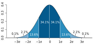
In statistics, the standard deviation is a measure of the amount of variation of the values of a variable about its mean. A low standard deviation indicates that the values tend to be close to the mean of the set, while a high standard deviation indicates that the values are spread out over a wider range. The standard deviation is commonly used in the determination of what constitutes an outlier and what does not.
The weighted arithmetic mean is similar to an ordinary arithmetic mean, except that instead of each of the data points contributing equally to the final average, some data points contribute more than others. The notion of weighted mean plays a role in descriptive statistics and also occurs in a more general form in several other areas of mathematics.
In statistics, maximum likelihood estimation (MLE) is a method of estimating the parameters of an assumed probability distribution, given some observed data. This is achieved by maximizing a likelihood function so that, under the assumed statistical model, the observed data is most probable. The point in the parameter space that maximizes the likelihood function is called the maximum likelihood estimate. The logic of maximum likelihood is both intuitive and flexible, and as such the method has become a dominant means of statistical inference.
In statistics, the Gauss–Markov theorem states that the ordinary least squares (OLS) estimator has the lowest sampling variance within the class of linear unbiased estimators, if the errors in the linear regression model are uncorrelated, have equal variances and expectation value of zero. The errors do not need to be normal, nor do they need to be independent and identically distributed. The requirement that the estimator be unbiased cannot be dropped, since biased estimators exist with lower variance. See, for example, the James–Stein estimator, ridge regression, or simply any degenerate estimator.
In statistics, the mean squared error (MSE) or mean squared deviation (MSD) of an estimator measures the average of the squares of the errors—that is, the average squared difference between the estimated values and the actual value. MSE is a risk function, corresponding to the expected value of the squared error loss. The fact that MSE is almost always strictly positive is because of randomness or because the estimator does not account for information that could produce a more accurate estimate. In machine learning, specifically empirical risk minimization, MSE may refer to the empirical risk, as an estimate of the true MSE.

In probability theory and statistics, the Rayleigh distribution is a continuous probability distribution for nonnegative-valued random variables. Up to rescaling, it coincides with the chi distribution with two degrees of freedom. The distribution is named after Lord Rayleigh.
In probability theory and statistics, a Gaussian process is a stochastic process, such that every finite collection of those random variables has a multivariate normal distribution. The distribution of a Gaussian process is the joint distribution of all those random variables, and as such, it is a distribution over functions with a continuous domain, e.g. time or space.
In statistics, a studentized residual is the dimensionless ratio resulting from the division of a residual by an estimate of its standard deviation, both expressed in the same units. It is a form of a Student's t-statistic, with the estimate of error varying between points.
In statistics, sometimes the covariance matrix of a multivariate random variable is not known but has to be estimated. Estimation of covariance matrices then deals with the question of how to approximate the actual covariance matrix on the basis of a sample from the multivariate distribution. Simple cases, where observations are complete, can be dealt with by using the sample covariance matrix. The sample covariance matrix (SCM) is an unbiased and efficient estimator of the covariance matrix if the space of covariance matrices is viewed as an extrinsic convex cone in Rp×p; however, measured using the intrinsic geometry of positive-definite matrices, the SCM is a biased and inefficient estimator. In addition, if the random variable has a normal distribution, the sample covariance matrix has a Wishart distribution and a slightly differently scaled version of it is the maximum likelihood estimate. Cases involving missing data, heteroscedasticity, or autocorrelated residuals require deeper considerations. Another issue is the robustness to outliers, to which sample covariance matrices are highly sensitive.

In statistics, ordinary least squares (OLS) is a type of linear least squares method for choosing the unknown parameters in a linear regression model by the principle of least squares: minimizing the sum of the squares of the differences between the observed dependent variable in the input dataset and the output of the (linear) function of the independent variable. Some sources consider OLS to be linear regression.
In statistics, the number of degrees of freedom is the number of values in the final calculation of a statistic that are free to vary.

In statistics, simple linear regression (SLR) is a linear regression model with a single explanatory variable. That is, it concerns two-dimensional sample points with one independent variable and one dependent variable and finds a linear function that, as accurately as possible, predicts the dependent variable values as a function of the independent variable. The adjective simple refers to the fact that the outcome variable is related to a single predictor.
In statistics, Cook's distance or Cook's D is a commonly used estimate of the influence of a data point when performing a least-squares regression analysis. In a practical ordinary least squares analysis, Cook's distance can be used in several ways: to indicate influential data points that are particularly worth checking for validity; or to indicate regions of the design space where it would be good to be able to obtain more data points. It is named after the American statistician R. Dennis Cook, who introduced the concept in 1977.
In statistics, generalized least squares (GLS) is a method used to estimate the unknown parameters in a linear regression model. It is used when there is a non-zero amount of correlation between the residuals in the regression model. GLS is employed to improve statistical efficiency and reduce the risk of drawing erroneous inferences, as compared to conventional least squares and weighted least squares methods. It was first described by Alexander Aitken in 1935.
In statistics, Mallows's, named for Colin Lingwood Mallows, is used to assess the fit of a regression model that has been estimated using ordinary least squares. It is applied in the context of model selection, where a number of predictor variables are available for predicting some outcome, and the goal is to find the best model involving a subset of these predictors. A small value of means that the model is relatively precise.
The topic of heteroskedasticity-consistent (HC) standard errors arises in statistics and econometrics in the context of linear regression and time series analysis. These are also known as heteroskedasticity-robust standard errors, Eicker–Huber–White standard errors, to recognize the contributions of Friedhelm Eicker, Peter J. Huber, and Halbert White.
In statistics, principal component regression (PCR) is a regression analysis technique that is based on principal component analysis (PCA). PCR is a form of reduced rank regression. More specifically, PCR is used for estimating the unknown regression coefficients in a standard linear regression model.
In statistics and in particular in regression analysis, leverage is a measure of how far away the independent variable values of an observation are from those of the other observations. High-leverage points, if any, are outliers with respect to the independent variables. That is, high-leverage points have no neighboring points in space, where is the number of independent variables in a regression model. This makes the fitted model likely to pass close to a high leverage observation. Hence high-leverage points have the potential to cause large changes in the parameter estimates when they are deleted i.e., to be influential points. Although an influential point will typically have high leverage, a high leverage point is not necessarily an influential point. The leverage is typically defined as the diagonal elements of the hat matrix.
The purpose of this page is to provide supplementary materials for the ordinary least squares article, reducing the load of the main article with mathematics and improving its accessibility, while at the same time retaining the completeness of exposition.


