Biostatistics (sometimes referred to as biometry) is a branch of statistics that applies statistical methods to a wide range of topics in the biological sciences, with a focus on clinical medicine and public health applications.[1] The field encompasses the design of experiments, the collection and analysis of experimental and observational data, and the interpretation of the results. It is closely related to medical statistics.
Biostatistical modeling forms an important part of numerous modern biological theories. Genetics studies, since its beginning, used statistical concepts to understand observed experimental results. Some genetics scientists even contributed with statistical advances with the development of methods and tools. Gregor Mendel started the genetics studies investigating genetics segregation patterns in families of peas and used statistics to explain the collected data. In the early 1900s, after the rediscovery of Mendel's Mendelian inheritance work, there were gaps in understanding between genetics and evolutionary Darwinism. Francis Galton tried to expand Mendel's discoveries with human data and proposed a different model with fractions of the heredity coming from each ancestral composing an infinite series. He called this the theory of "Law of Ancestral Heredity". His ideas were strongly disagreed by William Bateson, who followed Mendel's conclusions, that genetic inheritance were exclusively from the parents, half from each of them. This led to a vigorous debate between the biometricians, who supported Galton's ideas, as Raphael Weldon, Arthur Dukinfield Darbishire and Karl Pearson, and Mendelians, who supported Bateson's (and Mendel's) ideas, such as Charles Davenport and Wilhelm Johannsen. Later, biometricians could not reproduce Galton conclusions in different experiments, and Mendel's ideas prevailed. By the 1930s, models built on statistical reasoning had helped to resolve these differences and to produce the neo-Darwinian modern evolutionary synthesis.
Solving these differences also allowed to define the concept of population genetics and brought together genetics and evolution. The three leading figures in the establishment of population genetics and this synthesis all relied on statistics and developed its use in biology.
J. B. S. Haldane's book, The Causes of Evolution, reestablished natural selection as the premier mechanism of evolution by explaining it in terms of the mathematical consequences of Mendelian genetics. He also developed the theory of primordial soup.
In parallel to this overall development, the pioneering work of D'Arcy Thompson in On Growth and Form also helped to add quantitative discipline to biological study.
Despite the fundamental importance and frequent necessity of statistical reasoning, there may nonetheless have been a tendency among biologists to distrust or deprecate results which are not qualitatively apparent. One anecdote describes Thomas Hunt Morgan banning the Friden calculator from his department at Caltech, saying "Well, I am like a guy who is prospecting for gold along the banks of the Sacramento River in 1849. With a little intelligence, I can reach down and pick up big nuggets of gold. And as long as I can do that, I'm not going to let any people in my department waste scarce resources in placer mining."[4]
Research planning
Any research in life sciences is proposed to answer a scientific question we might have. To answer this question with a high certainty, we need accurate results. The correct definition of the main hypothesis and the research plan will reduce errors while taking a decision in understanding a phenomenon. The research plan might include the research question, the hypothesis to be tested, the experimental design, data collection methods, data analysis perspectives and costs involved. It is essential to carry the study based on the three basic principles of experimental statistics: randomization, replication, and local control.
Research question
The research question will define the objective of a study. The research will be headed by the question, so it needs to be concise, at the same time it is focused on interesting and novel topics that may improve science and knowledge and that field. To define the way to ask the scientific question, an exhaustive literature review might be necessary. So the research can be useful to add value to the scientific community.[5]
Hypothesis definition
Once the aim of the study is defined, the possible answers to the research question can be proposed, transforming this question into a hypothesis. The main propose is called null hypothesis (H0) and is usually based on a permanent knowledge about the topic or an obvious occurrence of the phenomena, sustained by a deep literature review. We can say it is the standard expected answer for the data under the situation in test. In general, HO assumes no association between treatments. On the other hand, the alternative hypothesis is the denial of HO. It assumes some degree of association between the treatment and the outcome. Although, the hypothesis is sustained by question research and its expected and unexpected answers.[5]
As an example, consider groups of similar animals (mice, for example) under two different diet systems. The research question would be: what is the best diet? In this case, H0 would be that there is no difference between the two diets in mice metabolism (H0: μ1 = μ2) and the alternative hypothesis would be that the diets have different effects over animals metabolism (H1: μ1 ≠ μ2).
The hypothesis is defined by the researcher, according to his/her interests in answering the main question. Besides that, the alternative hypothesis can be more than one hypothesis. It can assume not only differences across observed parameters, but their degree of differences (i.e. higher or shorter).
Sampling
Usually, a study aims to understand an effect of a phenomenon over a population. In biology, a population is defined as all the individuals of a given species, in a specific area at a given time. In biostatistics, this concept is extended to a variety of collections possible of study. Although, in biostatistics, a population is not only the individuals, but the total of one specific component of their organisms, as the whole genome, or all the sperm cells, for animals, or the total leaf area, for a plant, for example.
It is not possible to take the measures from all the elements of a population. Because of that, the sampling process is very important for statistical inference. Sampling is defined as to randomly get a representative part of the entire population, to make posterior inferences about the population. So, the sample might catch the most variability across a population.[6] The sample size is determined by several things, since the scope of the research to the resources available. In clinical research, the trial type, as inferiority, equivalence, and superiority is a key in determining sample size.[5]
Data collection methods must be considered in research planning, because it highly influences the sample size and experimental design.
Data collection varies according to the type of data. For qualitative data, collection can be done with structured questionnaires or by observation, considering presence or intensity of disease, using score criterion to categorize levels of occurrence.[8] For quantitative data, collection is done by measuring numerical information using instruments.
In agriculture and biology studies, yield data and its components can be obtained by metric measures. However, pest and disease injuries in plants are obtained by observation, considering score scales for levels of damage. Especially, in genetic studies, modern methods for data collection in field and laboratory should be considered, as high-throughput platforms for phenotyping and genotyping. These tools allow bigger experiments, while turn possible evaluate many plots in lower time than a human-based only method for data collection. Finally, all data collected of interest must be stored in an organized data frame for further analysis.
Data can be represented through tables or graphical representation, such as line charts, bar charts, histograms, scatter plot. Also, measures of central tendency and variability can be very useful to describe an overview of the data. Follow some examples:
Frequency tables
One type of table is the frequency table, which consists of data arranged in rows and columns, where the frequency is the number of occurrences or repetitions of data. Frequency can be:[9]
Absolute: represents the number of times that a determined value appear;
Relative: obtained by the division of the absolute frequency by the total number;
In the next example, we have the number of genes in ten operons of the same organism.
Genes = {2,3,3,4,5,3,3,3,3,4}
Genes number
Absolute frequency
Relative frequency
1
0
0
2
1
0.1
3
6
0.6
4
2
0.2
5
1
0.1
Line graph
Figure A: Line graph example. The birth rate in Brazil (2010–2016); Figure B: Bar chart example. The birth rate in Brazil for the December months from 2010 to 2016; Figure C: Example of Box Plot: number of glycines in the proteome of eight different organisms (A-H); Figure D: Example of a scatter plot.
Line graphs represent the variation of a value over another metric, such as time. In general, values are represented in the vertical axis, while the time variation is represented in the horizontal axis.[11]
Bar chart
A bar chart is a graph that shows categorical data as bars presenting heights (vertical bar) or widths (horizontal bar) proportional to represent values. Bar charts provide an image that could also be represented in a tabular format.[11]
In the bar chart example, we have the birth rate in Brazil for the December months from 2010 to 2016.[10] The sharp fall in December 2016 reflects the outbreak of Zika virus in the birth rate in Brazil.
Histograms
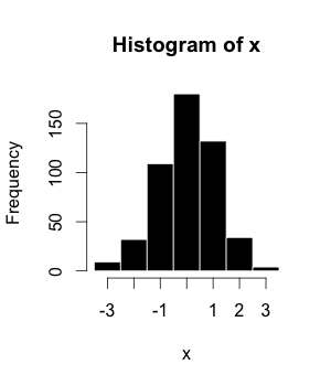
Example of a histogram.
The histogram (or frequency distribution) is a graphical representation of a dataset tabulated and divided into uniform or non-uniform classes. It was first introduced by Karl Pearson.[12]
Scatter plot
A scatter plot is a mathematical diagram that uses Cartesian coordinates to display values of a dataset. A scatter plot shows the data as a set of points, each one presenting the value of one variable determining the position on the horizontal axis and another variable on the vertical axis.[13] They are also called scatter graph, scatter chart, scattergram, or scatter diagram.[14]
Box plot is a method for graphically depicting groups of numerical data. The maximum and minimum values are represented by the lines, and the interquartile range (IQR) represent 25–75% of the data. Outliers may be plotted as circles.
Correlation coefficients
Although correlations between two different kinds of data could be inferred by graphs, such as scatter plot, it is necessary validate this though numerical information. For this reason, correlation coefficients are required. They provide a numerical value that reflects the strength of an association.[11]
Pearson correlation coefficient
Scatter diagram that demonstrates the Pearson correlation for different values of ρ.
Pearson correlation coefficient is a measure of association between two variables, X and Y. This coefficient, usually represented by ρ (rho) for the population and r for the sample, assumes values between −1 and 1, where ρ = 1 represents a perfect positive correlation, ρ = −1 represents a perfect negative correlation, and ρ = 0 is no linear correlation.[11]
It is used to make inferences[16] about an unknown population, by estimation and/or hypothesis testing. In other words, it is desirable to obtain parameters to describe the population of interest, but since the data is limited, it is necessary to make use of a representative sample in order to estimate them. With that, it is possible to test previously defined hypotheses and apply the conclusions to the entire population. The standard error of the mean is a measure of variability that is crucial to do inferences.[6]
Hypothesis testing is essential to make inferences about populations aiming to answer research questions, as settled in "Research planning" section. Authors defined four steps to be set:[6]
The hypothesis to be tested: as stated earlier, we have to work with the definition of a null hypothesis (H0), that is going to be tested, and an alternative hypothesis. But they must be defined before the experiment implementation.
Significance level and decision rule: A decision rule depends on the level of significance, or in other words, the acceptable error rate (α). It is easier to think that we define a critical value that determines the statistical significance when a test statistic is compared with it. So, α also has to be predefined before the experiment.
Experiment and statistical analysis: This is when the experiment is really implemented following the appropriate experimental design, data is collected and the more suitable statistical tests are evaluated.
Inference: Is made when the null hypothesis is rejected or not rejected, based on the evidence that the comparison of p-values and α brings. It is pointed that the failure to reject H0 just means that there is not enough evidence to support its rejection, but not that this hypothesis is true.
A confidence interval is a range of values that can contain the true real parameter value in given a certain level of confidence. The first step is to estimate the best-unbiased estimate of the population parameter. The upper value of the interval is obtained by the sum of this estimate with the multiplication between the standard error of the mean and the confidence level. The calculation of lower value is similar, but instead of a sum, a subtraction must be applied.[6]
Statistical considerations
Power and statistical error
When testing a hypothesis, there are two types of statistic errors possible: Type I error and Type II error.
The type I error or false positive is the incorrect rejection of a true null hypothesis
The significance level denoted by α is the type I error rate and should be chosen before performing the test. The type II error rate is denoted by β and statistical power of the test is 1 − β.
p-value
The p-value is the probability of obtaining results as extreme as or more extreme than those observed, assuming the null hypothesis (H0) is true. It is also called the calculated probability. It is common to confuse the p-value with the significance level (α), but, the α is a predefined threshold for calling significant results. If p is less than α, the null hypothesis (H0) is rejected.[17]
Multiple testing
In multiple tests of the same hypothesis, the probability of the occurrence of false positives(familywise error rate) increase and a strategy is needed to account for this occurrence. This is commonly achieved by using a more stringent threshold to reject null hypotheses. The Bonferroni correction defines an acceptable global significance level, denoted by α* and each test is individually compared with a value of α = α*/m. This ensures that the familywise error rate in all m tests, is less than or equal to α*. When m is large, the Bonferroni correction may be overly conservative. An alternative to the Bonferroni correction is to control the false discovery rate (FDR). The FDR controls the expected proportion of the rejected null hypotheses (the so-called discoveries) that are false (incorrect rejections). This procedure ensures that, for independent tests, the false discovery rate is at most q*. Thus, the FDR is less conservative than the Bonferroni correction and have more power, at the cost of more false positives.[18]
Mis-specification and robustness checks
The main hypothesis being tested (e.g., no association between treatments and outcomes) is often accompanied by other technical assumptions (e.g., about the form of the probability distribution of the outcomes) that are also part of the null hypothesis. When the technical assumptions are violated in practice, then the null may be frequently rejected even if the main hypothesis is true. Such rejections are said to be due to model mis-specification.[19] Verifying whether the outcome of a statistical test does not change when the technical assumptions are slightly altered (so-called robustness checks) is the main way of combating mis-specification.
Recent developments have made a large impact on biostatistics. Two important changes have been the ability to collect data on a high-throughput scale, and the ability to perform much more complex analysis using computational techniques. This comes from the development in areas as sequencing technologies, Bioinformatics and Machine learning (Machine learning in bioinformatics).
Use in high-throughput data
New biomedical technologies like microarrays, next-generation sequencers (for genomics) and mass spectrometry (for proteomics) generate enormous amounts of data, allowing many tests to be performed simultaneously.[20] Careful analysis with biostatistical methods is required to separate the signal from the noise. For example, a microarray could be used to measure many thousands of genes simultaneously, determining which of them have different expression in diseased cells compared to normal cells. However, only a fraction of genes will be differentially expressed.[21]
Multicollinearity often occurs in high-throughput biostatistical settings. Due to high intercorrelation between the predictors (such as gene expression levels), the information of one predictor might be contained in another one. It could be that only 5% of the predictors are responsible for 90% of the variability of the response. In such a case, one could apply the biostatistical technique of dimension reduction (for example via principal component analysis). Classical statistical techniques like linear or logistic regression and linear discriminant analysis do not work well for high dimensional data (i.e. when the number of observations n is smaller than the number of features or predictors p: n < p). As a matter of fact, one can get quite high R2-values despite very low predictive power of the statistical model. These classical statistical techniques (esp. least squares linear regression) were developed for low dimensional data (i.e. where the number of observations n is much larger than the number of predictors p: n >> p). In cases of high dimensionality, one should always consider an independent validation test set and the corresponding residual sum of squares (RSS) and R2 of the validation test set, not those of the training set.
Often, it is useful to pool information from multiple predictors together. For example, Gene Set Enrichment Analysis (GSEA) considers the perturbation of whole (functionally related) gene sets rather than of single genes.[22] These gene sets might be known biochemical pathways or otherwise functionally related genes. The advantage of this approach is that it is more robust: It is more likely that a single gene is found to be falsely perturbed than it is that a whole pathway is falsely perturbed. Furthermore, one can integrate the accumulated knowledge about biochemical pathways (like the JAK-STAT signaling pathway) using this approach.
Bioinformatics advances in databases, data mining, and biological interpretation
The development of biological databases enables storage and management of biological data with the possibility of ensuring access for users around the world. They are useful for researchers depositing data, retrieve information and files (raw or processed) originated from other experiments or indexing scientific articles, as PubMed. Another possibility is search for the desired term (a gene, a protein, a disease, an organism, and so on) and check all results related to this search. There are databases dedicated to SNPs (dbSNP), the knowledge on genes characterization and their pathways (KEGG) and the description of gene function classifying it by cellular component, molecular function and biological process (Gene Ontology).[23] In addition to databases that contain specific molecular information, there are others that are ample in the sense that they store information about an organism or group of organisms. As an example of a database directed towards just one organism, but that contains much data about it, is the Arabidopsis thaliana genetic and molecular database – TAIR.[24] Phytozome,[25] in turn, stores the assemblies and annotation files of dozen of plant genomes, also containing visualization and analysis tools. Moreover, there is an interconnection between some databases in the information exchange/sharing and a major initiative was the International Nucleotide Sequence Database Collaboration (INSDC)[26] which relates data from DDBJ,[27] EMBL-EBI,[28] and NCBI.[29]
Nowadays, increase in size and complexity of molecular datasets leads to use of powerful statistical methods provided by computer science algorithms which are developed by machine learning area. Therefore, data mining and machine learning allow detection of patterns in data with a complex structure, as biological ones, by using methods of supervised and unsupervised learning, regression, detection of clusters and association rule mining, among others.[23] To indicate some of them, self-organizing maps and k-means are examples of cluster algorithms; neural networks implementation and support vector machines models are examples of common machine learning algorithms.
Collaborative work among molecular biologists, bioinformaticians, statisticians and computer scientists is important to perform an experiment correctly, going from planning, passing through data generation and analysis, and ending with biological interpretation of the results.[23]
Use of computationally intensive methods
On the other hand, the advent of modern computer technology and relatively cheap computing resources have enabled computer-intensive biostatistical methods like bootstrapping and re-sampling methods.
In recent times, random forests have gained popularity as a method for performing statistical classification. Random forest techniques generate a panel of decision trees. Decision trees have the advantage that you can draw them and interpret them (even with a basic understanding of mathematics and statistics). Random Forests have thus been used for clinical decision support systems.[citation needed]
With new technologies and genetics knowledge, biostatistics are now also used for Systems medicine, which consists in a more personalized medicine. For this, is made an integration of data from different sources, including conventional patient data, clinico-pathological parameters, molecular and genetic data as well as data generated by additional new-omics technologies.[30]
Quantitative genetics
The study of population genetics and statistical genetics in order to link variation in genotype with a variation in phenotype. In other words, it is desirable to discover the genetic basis of a measurable trait, a quantitative trait, that is under polygenic control. A genome region that is responsible for a continuous trait is called a quantitative trait locus (QTL). The study of QTLs become feasible by using molecular markers and measuring traits in populations, but their mapping needs the obtaining of a population from an experimental crossing, like an F2 or recombinant inbred strains/lines (RILs). To scan for QTLs regions in a genome, a gene map based on linkage have to be built. Some of the best-known QTL mapping algorithms are Interval Mapping, Composite Interval Mapping, and Multiple Interval Mapping.[31]
However, QTL mapping resolution is impaired by the amount of recombination assayed, a problem for species in which it is difficult to obtain large offspring. Furthermore, allele diversity is restricted to individuals originated from contrasting parents, which limit studies of allele diversity when we have a panel of individuals representing a natural population.[32] For this reason, the genome-wide association study was proposed in order to identify QTLs based on linkage disequilibrium, that is the non-random association between traits and molecular markers. It was leveraged by the development of high-throughput SNP genotyping.[33]
In animal and plant breeding, the use of markers in selection aiming for breeding, mainly the molecular ones, collaborated to the development of marker-assisted selection. While QTL mapping is limited due resolution, GWAS does not have enough power when rare variants of small effect that are also influenced by environment. So, the concept of Genomic Selection (GS) arises in order to use all molecular markers in the selection and allow the prediction of the performance of candidates in this selection. The proposal is to genotype and phenotype a training population, develop a model that can obtain the genomic estimated breeding values (GEBVs) of individuals belonging to a genotype and but not phenotype population, called testing population.[34] This kind of study could also include a validation population, thinking in the concept of cross-validation, in which the real phenotype results measured in this population are compared with the phenotype results based on the prediction, what used to check the accuracy of the model.
As a summary, some points about the application of quantitative genetics are:
In biomedical research, this work can assist in finding candidates genealleles that can cause or influence predisposition to diseases in human genetics
Expression data
Studies for differential expression of genes from RNA-Seq data, as for RT-qPCR and microarrays, demands comparison of conditions. The goal is to identify genes which have a significant change in abundance between different conditions. Then, experiments are designed appropriately, with replicates for each condition/treatment, randomization and blocking, when necessary. In RNA-Seq, the quantification of expression uses the information of mapped reads that are summarized in some genetic unit, as exons that are part of a gene sequence. As microarray results can be approximated by a normal distribution, RNA-Seq counts data are better explained by other distributions. The first used distribution was the Poisson one, but it underestimate the sample error, leading to false positives. Currently, biological variation is considered by methods that estimate a dispersion parameter of a negative binomial distribution. Generalized linear models are used to perform the tests for statistical significance and as the number of genes is high, multiple tests correction have to be considered.[35] Some examples of other analysis on genomics data comes from microarray or proteomics experiments.[36][37] Often concerning diseases or disease stages.[38]
There are a lot of tools that can be used to do statistical analysis in biological data. Most of them are useful in other areas of knowledge, covering a large number of applications (alphabetical). Here are brief descriptions of some of them:
ASReml: Another software developed by VSNi[41] that can be used also in R environment as a package. It is developed to estimate variance components under a general linear mixed model using restricted maximum likelihood (REML). Models with fixed effects and random effects and nested or crossed ones are allowed. Gives the possibility to investigate different variance-covariance matrix structures.
CycDesigN:[42] A computer package developed by VSNi[41] that helps the researchers create experimental designs and analyze data coming from a design present in one of three classes handled by CycDesigN. These classes are resolvable, non-resolvable, partially replicated and crossover designs. It includes less used designs the Latinized ones, as t-Latinized design.[43]
Orange: A programming interface for high-level data processing, data mining and data visualization. Include tools for gene expression and genomics.[23]
R: An open source environment and programming language dedicated to statistical computing and graphics. It is an implementation of S language maintained by CRAN.[44] In addition to its functions to read data tables, take descriptive statistics, develop and evaluate models, its repository contains packages developed by researchers around the world. This allows the development of functions written to deal with the statistical analysis of data that comes from specific applications.[45] In the case of Bioinformatics, for example, there are packages located in the main repository (CRAN) and in others, as Bioconductor. It is also possible to use packages under development that are shared in hosting-services as GitHub.
SAS: A data analysis software widely used, going through universities, services and industry. Developed by a company with the same name (SAS Institute), it uses SAS language for programming.
PLA 3.0:[46] Is a biostatistical analysis software for regulated environments (e.g. drug testing) which supports Quantitative Response Assays (Parallel-Line, Parallel-Logistics, Slope-Ratio) and Dichotomous Assays (Quantal Response, Binary Assays). It also supports weighting methods for combination calculations and the automatic data aggregation of independent assay data.
Weka: A Java software for machine learning and data mining, including tools and methods for visualization, clustering, regression, association rule, and classification. There are tools for cross-validation, bootstrapping and a module of algorithm comparison. Weka also can be run in other programming languages as Perl or R.[23]
MyCalPharm: A software for pharmacology experiments, including Statistics Workshop. There are ten main topics that make up the module, each addresses an important aspect of statistics used in biological experiments - Data Features, Distribution of Data, Summary Statistics, Inferential Statistics, Choosing a Test, Sample Size, t-Test and Wilcoxon Test, ANOVA (Analysis of Variance), Correlation and Regression and Chi-Square Test.[47]
Scope and training programs
Almost all educational programmes in biostatistics are at postgraduate level. They are most often found in schools of public health, affiliated with schools of medicine, forestry, or agriculture, or as a focus of application in departments of statistics.
In the United States, where several universities have dedicated biostatistics departments, many other top-tier universities integrate biostatistics faculty into statistics or other departments, such as epidemiology. Thus, departments carrying the name "biostatistics" may exist under quite different structures. For instance, relatively new biostatistics departments have been founded with a focus on bioinformatics and computational biology, whereas older departments, typically affiliated with schools of public health, will have more traditional lines of research involving epidemiological studies and clinical trials as well as bioinformatics. In larger universities around the world, where both a statistics and a biostatistics department exist, the degree of integration between the two departments may range from the bare minimum to very close collaboration. In general, the difference between a statistics program and a biostatistics program is twofold: (i) statistics departments will often host theoretical/methodological research which are less common in biostatistics programs and (ii) statistics departments have lines of research that may include biomedical applications but also other areas such as industry (quality control), business and economics and biological areas other than medicine.
↑Szczech, Lynda Anne; Coladonato, Joseph A.; Owen, William F. (4 October 2002). "Key Concepts in Biostatistics: Using Statistics to Answer the Question "Is There a Difference?"". Seminars in Dialysis. 15 (5): 347–351. doi:10.1046/j.1525-139X.2002.00085.x. PMID12358639. S2CID30875225.
1234Forthofer, Ronald N.; Lee, Eun Sul (1995). Introduction to Biostatistics. A Guide to Design, Analysis, and Discovery. Academic Press. ISBN978-0-12-262270-0.
↑Benjamini, Y. & Hochberg, Y. Controlling the False Discovery Rate: A Practical and Powerful Approach to Multiple Testing. Journal of the Royal Statistical Society. Series B (Methodological) 57, 289–300 (1995).
↑Helen Causton; John Quackenbush; Alvis Brazma (2003). Statistical Analysis of Gene Expression Microarray Data. Wiley-Blackwell.
↑Terry Speed (2003). Microarray Gene Expression Data Analysis: A Beginner's Guide. Chapman & Hall/CRC.
↑Frank Emmert-Streib; Matthias Dehmer (2010). Medical Biostatistics for Complex Diseases. Wiley-Blackwell. ISBN978-3-527-32585-6.
↑Warren J. Ewens; Gregory R. Grant (2004). Statistical Methods in Bioinformatics: An Introduction. Springer.
↑Matthias Dehmer; Frank Emmert-Streib; Armin Graber; Armindo Salvador (2011). Applied Statistics for Network Biology: Methods in Systems Biology. Wiley-Blackwell. ISBN978-3-527-32750-8.
This page is based on this Wikipedia article Text is available under the CC BY-SA 4.0 license; additional terms may apply. Images, videos and audio are available under their respective licenses.