Bootstrapping is a procedure for estimating the distribution of an estimator by resampling (often with replacement) one's data or a model which is estimated from the data.[1] Bootstrapping assigns measures of accuracy (bias, variance, confidence intervals, prediction error, etc.) to sample estimates.[2][3] This technique allows estimation of the sampling distribution of almost any statistic using random sampling methods.[1]
Bootstrapping estimates the properties of an estimand (such as its variance) by measuring those properties when sampling from an approximating distribution. One standard choice for an approximating distribution is the empirical distribution function of the observed data. In the case where a set of observations can be assumed to be from an independent and identically distributed population, this can be implemented by constructing a number of resamples with replacement, of the observed data set (and of equal size to the observed data set). A key result in Efron's seminal paper that introduced the bootstrap[4] is the favorable performance of bootstrap methods using sampling with replacement compared to prior methods like the jackknife that sample without replacement. However, since its introduction, numerous variants on the bootstrap have been proposed, including methods that sample without replacement or that create bootstrap samples larger or smaller than the original data.
The bootstrap may also be used for constructing hypothesis tests.[5] It is often used as an alternative to statistical inference based on the assumption of a parametric model when that assumption is in doubt, or where parametric inference is impossible or requires complicated formulas for the calculation of standard errors.
History
The bootstrap[a] was first described by Bradley Efron in "Bootstrap methods: another look at the jackknife" (1979),[4] inspired by earlier work on the jackknife.[6][7][8] Improved estimates of the variance were developed later.[9][10] A Bayesian extension was developed in 1981.[11] The bias-corrected and accelerated () bootstrap was developed by Efron in 1987,[12] and the approximate bootstrap confidence interval (ABC, or approximate ) procedure in 1992.[13]
Approach
A sample is drawn from a population. From this sample, resamples are generated by drawing with replacement (orange). Data points that were drawn more than once (which happens for approx. 26.4% of data points) are shown in red and slightly offsetted. From the resamples, the statistic is calculated and, therefore, a histogram can be calculated to estimate the distribution of .
The basic idea of bootstrapping is that inference about a population from sample data (sample → population) can be modeled by resampling the sample data and performing inference about a sample from resampled data (resampled → sample).[14] As the population is unknown, the true error in a sample statistic against its population value is unknown. In bootstrap-resamples, the 'population' is in fact the sample, and this is known; hence the quality of inference of the 'true' sample from resampled data (resampled → sample) is measurable.
More formally, the bootstrap works by treating inference of the true probability distributionJ, given the original data, as being analogous to an inference of the empirical distribution Ĵ, given the resampled data. The accuracy of inferences regarding Ĵ using the resampled data can be assessed because we know Ĵ. If Ĵ is a reasonable approximation to J, then the quality of inference on J can in turn be inferred.
As an example, assume we are interested in the average (or mean) height of people worldwide. We cannot measure all the people in the global population, so instead, we sample only a tiny part of it, and measure that. Assume the sample is of size N; that is, we measure the heights of N individuals. From that single sample, only one estimate of the mean can be obtained. In order to reason about the population, we need some sense of the variability of the mean that we have computed. The simplest bootstrap method involves taking the original data set of heights, and, using a computer, sampling from it to form a new sample (called a 'resample' or bootstrap sample) that is also of sizeN. The bootstrap sample is taken from the original by using sampling with replacement (e.g. we might 'resample' 5 times from [1,2,3,4,5] and get [2,5,4,4,1]), so, assuming N is sufficiently large, for all practical purposes there is virtually zero probability that it will be identical to the original "real" sample. This process is repeated a large number of times (typically 1,000 or 10,000 times), and for each of these bootstrap samples, we compute its mean (each of these is called a "bootstrap estimate"). We now can create a histogram of bootstrap means. This histogram provides an estimate of the shape of the distribution of the sample mean from which we can answer questions about how much the mean varies across samples. (The method here, described for the mean, can be applied to almost any other statistic or estimator.)
A great advantage of bootstrap is its simplicity. It is a straightforward way to derive estimates of standard errors and confidence intervals for complex estimators of the distribution, such as percentile points, proportions, Odds ratio, and correlation coefficients. However, despite its simplicity, bootstrapping can be applied to complex sampling designs (e.g. for population divided into s strata with ns observations per strata, one example of which is a dose-response experiment, where bootstrapping can be applied for each stratum).[15] Bootstrap is also an appropriate way to control and check the stability of the results. Although for most problems it is impossible to know the true confidence interval, bootstrap is asymptotically more accurate than the standard intervals obtained using sample variance and assumptions of normality.[16] Bootstrapping is also a convenient method that avoids the cost of repeating the experiment to get other groups of sample data.
Disadvantages
Bootstrapping depends heavily on the estimator used and, though simple, naive use of bootstrapping will not always yield asymptotically valid results and can lead to inconsistency.[17] Although bootstrapping is (under some conditions) asymptotically consistent, it does not provide general finite-sample guarantees. The result may depend on the representative sample. The apparent simplicity may conceal the fact that important assumptions are being made when undertaking the bootstrap analysis (e.g. independence of samples or large enough of a sample size) where these would be more formally stated in other approaches. Also, bootstrapping can be time-consuming and there are not many available software for bootstrapping as it is difficult to automate using traditional statistical computer packages.[15]
Recommendations
Scholars have recommended more bootstrap samples as available computing power has increased. If the results may have substantial real-world consequences, then one should use as many samples as is reasonable, given available computing power and time. Increasing the number of samples cannot increase the amount of information in the original data; it can only reduce the effects of random sampling errors which can arise from a bootstrap procedure itself. Moreover, there is evidence that numbers of samples greater than 100 lead to negligible improvements in the estimation of standard errors.[18] In fact, according to the original developer of the bootstrapping method, even setting the number of samples at 50 is likely to lead to fairly good standard error estimates.[19]
Adèr et al. recommend the bootstrap procedure for the following situations:[20]
When the theoretical distribution of a statistic of interest is complicated or unknown. Since the bootstrapping procedure is distribution-independent it provides an indirect method to assess the properties of the distribution underlying the sample and the parameters of interest that are derived from this distribution.
When the sample size is insufficient for straightforward statistical inference. If the underlying distribution is well-known, bootstrapping provides a way to account for the distortions caused by the specific sample that may not be fully representative of the population.
When power calculations have to be performed, and a small pilot sample is available. Most power and sample size calculations are heavily dependent on the standard deviation of the statistic of interest. If the estimate used is incorrect, the required sample size will also be wrong. One method to get an impression of the variation of the statistic is to use a small pilot sample and perform bootstrapping on it to get impression of the variance.
However, Athreya has shown[21] that if one performs a naive bootstrap on the sample mean when the underlying population lacks a finite variance (for example, a power law distribution), then the bootstrap distribution will not converge to the same limit as the sample mean. As a result, confidence intervals on the basis of a Monte Carlo simulation of the bootstrap could be misleading. Athreya states that "Unless one is reasonably sure that the underlying distribution is not heavy tailed, one should hesitate to use the naive bootstrap".
In univariate problems, it is usually acceptable to resample the individual observations with replacement ("case resampling" below) unlike subsampling, in which resampling is without replacement and is valid under much weaker conditions compared to the bootstrap. In small samples, a parametric bootstrap approach might be preferred. For other problems, a smooth bootstrap will likely be preferred.
For regression problems, various other alternatives are available.[2]
Case resampling
The bootstrap is generally useful for estimating the distribution of a statistic (e.g. mean, variance) without using normality assumptions (as required, e.g., for a z-statistic or a t-statistic). In particular, the bootstrap is useful when there is no analytical form or an asymptotic theory (e.g., an applicable central limit theorem) to help estimate the distribution of the statistics of interest. This is because bootstrap methods can apply to most random quantities, e.g., the ratio of variance and mean. There are at least two ways of performing case resampling.
The Monte Carlo algorithm for case resampling is quite simple. First, we resample the data with replacement, and the size of the resample must be equal to the size of the original data set. Then the statistic of interest is computed from the resample from the first step. We repeat this routine many times to get a more precise estimate of the Bootstrap distribution of the statistic.[2]
The 'exact' version for case resampling is similar, but we exhaustively enumerate every possible resample of the data set. This can be computationally expensive as there are a total of different resamples, where n is the size of the data set. Thus for n=5,10,20,30 there are 126, 92378, 6.89×10¹⁰ and 5.91×10¹⁶ different resamples respectively.[22]
Estimating the distribution of sample mean
Consider a coin-flipping experiment. We flip the coin and record whether it lands heads or tails. Let X = x1, x2, …, x10 be 10 observations from the experiment. xi = 1 if the i th flip lands heads, and 0 otherwise. By invoking the assumption that the average of the coin flips is normally distributed, we can use the t-statistic to estimate the distribution of the sample mean,
Such a normality assumption can be justified either as an approximation of the distribution of each individual coin flip or as an approximation of the distribution of the average of a large number of coin flips. The former is a poor approximation because the true distribution of the coin flips is Bernoulli instead of normal. The latter is a valid approximation in infinitely large samples due to the central limit theorem.
However, if we are not ready to make such a justification, then we can use the bootstrap instead. Using case resampling, we can derive the distribution of . We first resample the data to obtain a bootstrap resample. An example of the first resample might look like this X1* = x2, x1, x10, x10, x3, x4, x6, x7, x1, x9. There are some duplicates since a bootstrap resample comes from sampling with replacement from the data. Also the number of data points in a bootstrap resample is equal to the number of data points in our original observations. Then we compute the mean of this resample and obtain the first bootstrap mean: μ1*. We repeat this process to obtain the second resample X2* and compute the second bootstrap mean μ2*. If we repeat this 100 times, then we have μ1*, μ2*, ..., μ100*. This represents an empirical bootstrap distribution of sample mean. From this empirical distribution, one can derive a bootstrap confidence interval for the purpose of hypothesis testing.
Regression
In regression problems, case resampling refers to the simple scheme of resampling individual cases – often rows of a data set. For regression problems, as long as the data set is fairly large, this simple scheme is often acceptable.[citation needed] However, the method is open to criticism[citation needed].[15]
In regression problems, the explanatory variables are often fixed, or at least observed with more control than the response variable. Also, the range of the explanatory variables defines the information available from them. Therefore, to resample cases means that each bootstrap sample will lose some information. As such, alternative bootstrap procedures should be considered.
Bayesian bootstrap
Bootstrapping can be interpreted in a Bayesian framework using a scheme that creates new data sets through reweighting the initial data. Given a set of data points, the weighting assigned to data point in a new data set is , where is a low-to-high ordered list of uniformly distributed random numbers on , preceded by 0 and succeeded by 1. The distributions of a parameter inferred from considering many such data sets are then interpretable as posterior distributions on that parameter.[23]
Smooth bootstrap
Under this scheme, a small amount of (usually normally distributed) zero-centered random noise is added onto each resampled observation. This is equivalent to sampling from a kernel density estimate of the data. Assume K to be a symmetric kernel density function with unit variance. The standard kernel estimator of is
Based on the assumption that the original data set is a realization of a random sample from a distribution of a specific parametric type, in this case a parametric model is fitted by parameter θ, often by maximum likelihood, and samples of random numbers are drawn from this fitted model. Usually the sample drawn has the same sample size as the original data. Then the estimate of original function F can be written as . This sampling process is repeated many times as for other bootstrap methods. Considering the centered sample mean in this case, the random sample original distribution function is replaced by a bootstrap random sample with function , and the probability distribution of is approximated by that of , where , which is the expectation corresponding to .[25] The use of a parametric model at the sampling stage of the bootstrap methodology leads to procedures which are different from those obtained by applying basic statistical theory to inference for the same model[citation needed].
Resampling residuals
Another approach to bootstrapping in regression problems is to resample residuals. The method proceeds as follows.
Fit the model and retain the fitted values and the residuals .
For each pair, (xi, yi), in which xi is the (possibly multivariate) explanatory variable, add a randomly resampled residual, , to the fitted value . In other words, create synthetic response variables where j is selected randomly from the list (1, ..., n) for every i.
Refit the model using the fictitious response variables , and retain the quantities of interest (often the parameters, , estimated from the synthetic ).
Repeat steps 2 and 3 a large number of times.
This scheme has the advantage that it retains the information in the explanatory variables. However, a question arises as to which residuals to resample. Raw residuals are one option; another is studentized residuals (in linear regression). Although there are arguments in favor of using studentized residuals; in practice, it often makes little difference, and it is easy to compare the results of both schemes.
Gaussian process regression bootstrap
When data are temporally correlated, straightforward bootstrapping destroys the inherent correlations. This method uses Gaussian process regression (GPR) to fit a probabilistic model from which replicates may then be drawn. GPR is a Bayesian non-linear regression method. A Gaussian process (GP) is a collection of random variables, any finite number of which have a joint Gaussian (normal) distribution. A GP is defined by a mean function and a covariance function, which specify the mean vectors and covariance matrices for each finite collection of the random variables.[26]
Regression model:
is a noise term.
Gaussian process prior:
For any finite collection of variables, x1,...,xn, the function outputs are jointly distributed according to a multivariate Gaussian with mean and covariance matrix
Assume Then ,
where , and is the standard Kronecker delta function.[26]
Gaussian process posterior:
According to GP prior, we can get
,
where and
Let x1*,...,xs* be another finite collection of variables, it's obvious that
,
where , ,
According to the equations above, the outputs y are also jointly distributed according to a multivariate Gaussian. Thus,
The wild bootstrap, proposed originally by Wu (1986),[27] is suited when the model exhibits heteroskedasticity. The idea is, as the residual bootstrap, to leave the regressors at their sample value, but to resample the response variable based on the residuals values. That is, for each replicate, one computes a new based on
so the residuals are randomly multiplied by a random variable with mean 0 and variance 1. For most distributions of (but not Mammen's), this method assumes that the 'true' residual distribution is symmetric and can offer advantages over simple residual sampling for smaller sample sizes. Different forms are used for the random variable , such as
The block bootstrap is used when the data, or the errors in a model, are correlated. In this case, a simple case or residual resampling will fail, as it is not able to replicate the correlation in the data. The block bootstrap tries to replicate the correlation by resampling inside blocks of data (see Blocking (statistics)). The block bootstrap has been used mainly with data correlated in time (i.e. time series) but can also be used with data correlated in space, or among groups (so-called cluster data).
Time series: Simple block bootstrap
In the (simple) block bootstrap, the variable of interest is split into non-overlapping blocks.
Time series: Moving block bootstrap
In the moving block bootstrap, introduced by Künsch (1989),[29] data is split into n−b+1 overlapping blocks of length b: Observation 1 to b will be block 1, observation 2 to b+1 will be block 2, etc. Then from these n−b+1 blocks, n/b blocks will be drawn at random with replacement. Then aligning these n/b blocks in the order they were picked, will give the bootstrap observations.
This bootstrap works with dependent data, however, the bootstrapped observations will not be stationary anymore by construction. But, it was shown that varying randomly the block length can avoid this problem.[30] This method is known as the stationary bootstrap. Other related modifications of the moving block bootstrap are the Markovian bootstrap and a stationary bootstrap method that matches subsequent blocks based on standard deviation matching.
Time series: Maximum entropy bootstrap
Vinod (2006),[31] presents a method that bootstraps time series data using maximum entropy principles satisfying the Ergodic theorem with mean-preserving and mass-preserving constraints. There is an R package, meboot,[32] that utilizes the method, which has applications in econometrics and computer science.
Cluster data: block bootstrap
Cluster data describes data where many observations per unit are observed. This could be observing many firms in many states or observing students in many classes. In such cases, the correlation structure is simplified, and one does usually make the assumption that data is correlated within a group/cluster, but independent between groups/clusters. The structure of the block bootstrap is easily obtained (where the block just corresponds to the group), and usually only the groups are resampled, while the observations within the groups are left unchanged. Cameron et al. (2008) discusses this for clustered errors in linear regression.[33]
Methods for improving computational efficiency
The bootstrap is a powerful technique although may require substantial computing resources in both time and memory. Some techniques have been developed to reduce this burden. They can generally be combined with many of the different types of Bootstrap schemes and various choices of statistics.
Parallel processing
Most bootstrap methods are embarrassingly parallel algorithms. That is, the statistic of interest for each bootstrap sample does not depend on other bootstrap samples. Such computations can therefore be performed on separate CPUs or compute nodes with the results from the separate nodes eventually aggregated for final analysis.
Poisson bootstrap
The nonparametric bootstrap samples items from a list of size n with counts drawn from a multinomial distribution. If denotes the number times element i is included in a given bootstrap sample, then each is distributed as a binomial distribution with n trials and mean 1, but is not independent of for .
The Poisson bootstrap instead draws samples assuming all 's are independently and identically distributed as Poisson variables with mean 1. The rationale is that the limit of the binomial distribution is Poisson:
The Poisson bootstrap had been proposed by Hanley and MacGibbon as potentially useful for non-statisticians using software like SAS and SPSS, which lacked the bootstrap packages of R and S-Plus programming languages.[34] The same authors report that for large enough n, the results are relatively similar to the nonparametric bootstrap estimates but go on to note the Poisson bootstrap has seen minimal use in applications.
Another proposed advantage of the Poisson bootstrap is the independence of the makes the method easier to apply for large datasets that must be processed as streams.[35]
A way to improve on the Poisson bootstrap, termed "sequential bootstrap", is by taking the first samples so that the proportion of unique values is ≈0.632 of the original sample size n. This provides a distribution with main empirical characteristics being within a distance of .[36] Empirical investigation has shown this method can yield good results.[37] This is related to the reduced bootstrap method.[38]
Bag of Little Bootstraps
For massive data sets, it is often computationally prohibitive to hold all the sample data in memory and resample from the sample data. The Bag of Little Bootstraps (BLB)[39] provides a method of pre-aggregating data before bootstrapping to reduce computational constraints. This works by partitioning the data set into equal-sized buckets and aggregating the data within each bucket. This pre-aggregated data set becomes the new sample data over which to draw samples with replacement. This method is similar to the Block Bootstrap, but the motivations and definitions of the blocks are very different. Under certain assumptions, the sample distribution should approximate the full bootstrapped scenario. One constraint is the number of buckets where and the authors recommend usage of as a general solution.
Choice of statistic
The bootstrap distribution of a point estimator of a population parameter has been used to produce a bootstrapped confidence interval for the parameter's true value if the parameter can be written as a function of the population's distribution.
A Bayesian point estimator and a maximum-likelihood estimator have good performance when the sample size is infinite, according to asymptotic theory. For practical problems with finite samples, other estimators may be preferable. Asymptotic theory suggests techniques that often improve the performance of bootstrapped estimators; the bootstrapping of a maximum-likelihood estimator may often be improved using transformations related to pivotal quantities.[40]
Deriving confidence intervals from the bootstrap distribution
The bootstrap distribution of a parameter-estimator is often used to calculate confidence intervals for its population-parameter.[2] A variety of methods for constructing the confidence intervals have been proposed, although there is disagreement which method is the best.
Desirable properties
The survey of bootstrap confidence interval methods of DiCiccio and Efron and consequent discussion lists several desired properties of confidence intervals, which generally are not all simultaneously met.
Transformation invariant - the confidence intervals from bootstrapping transformed data (e.g., by taking the logarithm) would ideally be the same as transforming the confidence intervals from bootstrapping the untransformed data.
Confidence intervals should be valid or consistent, i.e., the probability a parameter is in a confidence interval with nominal level should be equal to or at least converge in probability to . The latter criteria is both refined and expanded using the framework of Hall.[41] The refinements are to distinguish between methods based on how fast the true coverage probability approaches the nominal value, where a method is (using DiCiccio and Efron's terminology) first-order accurate if the error term in the approximation is and second-order accurate if the error term is . In addition, methods are distinguished by the speed with which the estimated bootstrap critical point converges to the true (unknown) point, and a method is second-order correct when this rate is .
Gleser in the discussion of the paper argues that a limitation of the asymptotic descriptions in the previous bullet is that the terms are not necessarily uniform in the parameters or true distribution.
Bias, asymmetry, and confidence intervals
Bias: The bootstrap distribution and the sample may disagree systematically, in which case bias may occur.
If the bootstrap distribution of an estimator is symmetric, then percentile confidence-interval are often used; such intervals are appropriate especially for median-unbiased estimators of minimum risk (with respect to an absoluteloss function). Bias in the bootstrap distribution will lead to bias in the confidence interval.
Otherwise, if the bootstrap distribution is non-symmetric, then percentile confidence intervals are often inappropriate.
Methods for bootstrap confidence intervals
There are several methods for constructing confidence intervals from the bootstrap distribution of a real parameter:
Basic bootstrap,[40] also known as the Reverse Percentile Interval.[42] The basic bootstrap is a simple scheme to construct the confidence interval: one simply takes the empirical quantiles from the bootstrap distribution of the parameter (see Davison and Hinkley 1997, equ. 5.6 p.194):
where denotes the percentile of the bootstrapped coefficients .
Percentile bootstrap. The percentile bootstrap proceeds in a similar way to the basic bootstrap, using percentiles of the bootstrap distribution, but with a different formula (note the inversion of the left and right quantiles):
where denotes the percentile of the bootstrapped coefficients .
See Davison and Hinkley (1997, equ. 5.18 p.203) and Efron and Tibshirani (1993, equ 13.5 p.171).
This method can be applied to any statistic. It will work well in cases where the bootstrap distribution is symmetrical and centered on the observed statistic[43] and where the sample statistic is median-unbiased and has maximum concentration (or minimum risk with respect to an absolute value loss function). When working with small sample sizes (i.e., less than 50), the basic / reversed percentile and percentile confidence intervals for (for example) the variance statistic will be too narrow. So that with a sample of 20 points, 90% confidence interval will include the true variance only 78% of the time.[44] The basic / reverse percentile confidence intervals are easier to justify mathematically[45][42] but they are less accurate in general than percentile confidence intervals, and some authors discourage their use.[42]
Studentized bootstrap. The studentized bootstrap, also called bootstrap-t, is computed analogously to the standard confidence interval, but replaces the quantiles from the normal or student approximation by the quantiles from the bootstrap distribution of the Student's t-test (see Davison and Hinkley 1997, equ. 5.7 p.194 and Efron and Tibshirani 1993 equ 12.22, p.160):
where denotes the percentile of the bootstrapped Student's t-test, and is the estimated standard error of the coefficient in the original model.
The studentized test enjoys optimal properties as the statistic that is bootstrapped is pivotal (i.e. it does not depend on nuisance parameters as the t-test follows asymptotically a N(0,1) distribution), unlike the percentile bootstrap.
Bias-corrected bootstrap – adjusts for bias in the bootstrap distribution.
Accelerated bootstrap – The bias-corrected and accelerated (BCa) bootstrap, by Efron (1987),[12] adjusts for both bias and skewness in the bootstrap distribution. This approach is accurate in a wide variety of settings, has reasonable computation requirements, and produces reasonably narrow intervals.[12]
Efron and Tibshirani[2] suggest the following algorithm for comparing the means of two independent samples: Let be a random sample from distribution F with sample mean and sample variance . Let be another, independent random sample from distribution G with mean and variance
Calculate the test statistic
Create two new data sets whose values are and where is the mean of the combined sample.
Draw a random sample () of size with replacement from and another random sample () of size with replacement from .
Calculate the test statistic
Repeat 3 and 4 times (e.g. ) to collect values of the test statistic.
Estimate the p-value as where when condition is true and 0 otherwise.
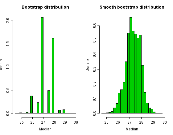
The bootstrap distribution for Newcomb's data appears below. We can reduce the discreteness of the bootstrap distribution by adding a small amount of random noise to each bootstrap sample. A conventional choice is to add noise with a standard deviation of for a sample size n; this noise is often drawn from a Student-t distribution with n-1 degrees of freedom.[47] This results in an approximately-unbiased estimator for the variance of the sample mean.[48] This means that samples taken from the bootstrap distribution will have a variance which is, on average, equal to the variance of the total population.
Histograms of the bootstrap distribution and the smooth bootstrap distribution appear below. The bootstrap distribution of the sample-median has only a small number of values. The smoothed bootstrap distribution has a richer support. However, note that whether the smoothed or standard bootstrap procedure is favorable is case-by-case and is shown to depend on both the underlying distribution function and on the quantity being estimated.[49]
In this example, the bootstrapped 95% (percentile) confidence-interval for the population median is (26, 28.5), which is close to the interval for (25.98, 28.46) for the smoothed bootstrap.
the jackknife procedure, used to estimate biases of sample statistics and to estimate variances, and
cross-validation, in which the parameters (e.g., regression weights, factor loadings) that are estimated in one subsample are applied to another subsample.
Bootstrap aggregating (bagging) is a meta-algorithm based on averaging model predictions obtained from models trained on multiple bootstrap samples.
In situations where an obvious statistic can be devised to measure a required characteristic using only a small number, r, of data items, a corresponding statistic based on the entire sample can be formulated. Given an r-sample statistic, one can create an n-sample statistic by something similar to bootstrapping (taking the average of the statistic over all subsamples of size r). This procedure is known to have certain good properties and the result is a U-statistic. The sample mean and sample variance are of this form, for r=1 and r=2.
Asymptotic theory
The bootstrap has under certain conditions desirable asymptotic properties. The asymptotic properties most often described are weak convergence / consistency of the sample paths of the bootstrap empirical process and the validity of confidence intervals derived from the bootstrap. This section describes the convergence of the empirical bootstrap.
Stochastic convergence
This paragraph summarizes more complete descriptions of stochastic convergence in van der Vaart and Wellner[50] and Kosorok.[51] The bootstrap defines a stochastic process, a collection of random variables indexed by some set , where is typically the real line () or a family of functions. Processes of interest are those with bounded sample paths, i.e., sample paths in L-infinity (), the set of all uniformly boundedfunctions from to . When equipped with the uniform distance, is a metric space, and when , two subspaces of are of particular interest, , the space of all continuous functions from to the unit interval [0,1], and , the space of all cadlag functions from to [0,1]. This is because contains the distribution functions for all continuous random variables, and contains the distribution functions for all random variables. Statements about the consistency of the bootstrap are statements about the convergence of the sample paths of the bootstrap process as random elements of the metric space or some subspace thereof, especially or .
Consistency
Horowitz in a recent review[1] defines consistency as: the bootstrap estimator is consistent [for a statistic ] if, for each , converges in probability to 0 as , where is the empirical distribution of the original sample, is the true but unknown distribution of the statistic, is the asymptotic distribution function of , and is the indexing variable in the distribution function, i.e., . This is sometimes more specifically called consistency relative to the Kolmogorov-Smirnov distance.[52]
Horowitz goes on to recommend using a theorem from Mammen[53] that provides easier to check necessary and sufficient conditions for consistency for statistics of a certain common form. In particular, let be the random sample. If for a sequence of numbers and , then the bootstrap estimate of the cumulative distribution function estimates the empirical cumulative distribution function if and only if converges in distribution to the standard normal distribution.
Strong consistency
Convergence in (outer) probability as described above is also called weak consistency. It can also be shown with slightly stronger assumptions, that the bootstrap is strongly consistent, where convergence in (outer) probability is replaced by convergence (outer) almost surely. When only one type of consistency is described, it is typically weak consistency. This is adequate for most statistical applications since it implies confidence bands derived from the bootstrap are asymptotically valid.[51]
Showing consistency using the central limit theorem
In simpler cases, it is possible to use the central limit theorem directly to show the consistency of the bootstrap procedure for estimating the distribution of the sample mean.
Specifically, let us consider independent identically distributed random variables with and for each . Let . In addition, for each , conditional on , let be independent random variables with distribution equal to the empirical distribution of . This is the sequence of bootstrap samples.
Then it can be shown that where represents probability conditional on , , , and .
↑Lehmann E.L. (1992) "Introduction to Neyman and Pearson (1933) On the Problem of the Most Efficient Tests of Statistical Hypotheses". In: Breakthroughs in Statistics, Volume 1, (Eds Kotz, S., Johnson, N.L.), Springer-Verlag. ISBN 0-387-94037-5 (followed by reprinting of the paper).
↑Efron, B., Rogosa, D., & Tibshirani, R. (2004). Resampling methods of estimation. In N.J. Smelser, & P.B. Baltes (Eds.). International Encyclopedia of the Social & Behavioral Sciences (pp. 13216–13220). New York, NY: Elsevier.
↑Dekking, Frederik Michel; Kraaikamp, Cornelis; Lopuhaä, Hendrik Paul; Meester, Ludolf Erwin (2005). A modern introduction to probability and statistics: understanding why and how. London: Springer. ISBN978-1-85233-896-1. OCLC262680588.
↑Vinod, HD (2006). "Maximum entropy ensembles for time series inference in economics". Journal of Asian Economics. 17 (6): 955–978. doi:10.1016/j.asieco.2006.09.001.
↑Jiménez-Gamero, María Dolores; Muñoz-García, Joaquín; Pino-Mejías, Rafael (2004). "Reduced bootstrap for the median". Statistica Sinica. 14 (4): 1179–1198. JSTOR24307226.
↑Kleiner, A; Talwalkar, A; Sarkar, P; Jordan, M. I. (2014). "A scalable bootstrap for massive data". Journal of the Royal Statistical Society, Series B (Statistical Methodology). 76 (4): 795–816. arXiv:1112.5016. doi:10.1111/rssb.12050. ISSN1369-7412. S2CID3064206.
123Hesterberg, Tim C (2014). "What Teachers Should Know about the Bootstrap: Resampling in the Undergraduate Statistics Curriculum". arXiv:1411.5279 [stat.OT].
↑Efron, B. (1982). The jackknife, the bootstrap, and other resampling plans. Vol.38. Society of Industrial and Applied Mathematics CBMS-NSF Monographs. ISBN0-89871-179-7.
↑Rice, John. Mathematical Statistics and Data Analysis (2ed.). p.272. "Although this direct equation of quantiles of the bootstrap sampling distribution with confidence limits may seem initially appealing, it’s rationale is somewhat obscure."
↑Mammen E (1992). When Does Bootstrap Work?: Aysmptotic Results and Simulations. Lecture Notes in Statistics. Vol.57. New York: Springer-Verlag. ISBN978-0-387-97867-3.
Efron B (1982). The Jackknife, the Bootstrap, and Other Resampling Plans. Society of Industrial and Applied Mathematics CBMS-NSF Monographs. Vol.38. Philadelphia, US: Society for Industrial and Applied Mathematics.
Mooney CZ, Duval RD (1993). Bootstrapping: A Nonparametric Approach to Statistical Inference. Sage University Paper Series on Quantitative Applications in the Social Sciences. Vol.07–095. Newbury Park, US: Sage.
Wright D, London K, Field AP (2011). "Using bootstrap estimation and the plug-in principle for clinical psychology data". Journal of Experimental Psychopathology. 2 (2): 252–270. doi:10.5127/jep.013611.
Gong G (1986). "Cross-validation, the jackknife, and the bootstrap: Excess error estimation in forward logistic regression". Journal of the American Statistical Association. 81 (393): 108–113. Bibcode:1986JASA...81..108G. doi:10.1080/01621459.1986.10478245.
↑Other names that Efron's colleagues suggested for the "bootstrap" method were: Swiss Army Knife, Meat Axe, Swan-Dive, Jack-Rabbit, and Shotgun.[4]
This page is based on this Wikipedia article Text is available under the CC BY-SA 4.0 license; additional terms may apply. Images, videos and audio are available under their respective licenses.