Numeric quantity representing the center of a collection of numbers
This article is about quantifying the concept of "typical value". For other uses, see Mean (disambiguation).For broader coverage of this topic, see Average.For the state of being mean or cruel, see Meanness.
A mean is a quantity representing the "center" of a collection of numbers and is intermediate to the extreme values of the set of numbers.[1] There are several kinds of means (or "measures of central tendency") in mathematics, especially in statistics. Each attempts to summarize or typify a given group of data, illustrating the magnitude and sign of the data set. Which of these measures is most illuminating depends on what is being measured, and on context and purpose.[2]
The arithmetic mean, also known as "arithmetic average", is the sum of the values divided by the number of values. The arithmetic mean of a set of numbers x1, x2, ..., xn is typically denoted using an overhead bar, .[note 1] If the numbers are from observing a sample of a larger group, the arithmetic mean is termed the sample mean () to distinguish it from the group mean (or expected value) of the underlying distribution, denoted or .[note 2][3]
In mathematics, the three classical Pythagorean means are the arithmetic mean (AM), the geometric mean (GM), and the harmonic mean (HM). These means were studied with proportions by Pythagoreans and later generations of Greek mathematicians[4] because of their importance in geometry and music.
The arithmetic mean (or simply mean or average) of a list of numbers, is the sum of all of the numbers divided by their count. Similarly, the mean of a sample , usually denoted by , is the sum of the sampled values divided by the number of items in the sample.
For example, the arithmetic mean of five values: 4, 36, 45, 50, 75 is:
Geometric mean (GM)
The geometric mean is an average that is useful for sets of positive numbers, that are interpreted according to their product (as is the case with rates of growth) and not their sum (as is the case with the arithmetic mean):[1]
For example, the geometric mean of five values: 4, 36, 45, 50, 75 is:
Harmonic mean (HM)
The harmonic mean is an average which is useful for sets of numbers which are defined in relation to some unit, as in the case of speed (i.e., distance per unit of time):
For example, the harmonic mean of the five values: 4, 36, 45, 50, 75 is
If we have five pumps that can empty a tank of a certain size in respectively 4, 36, 45, 50, and 75 minutes, then the harmonic mean of tells us that these five different pumps working together will pump at the same rate as five pumps that can each empty the tank in minutes.
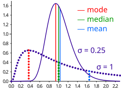
Comparison of the arithmetic mean, median, and mode of two skewed (log-normal) distributionsGeometric visualization of the mode, median and mean of an arbitrary probability density function
In descriptive statistics, the mean may be confused with the median, mode or mid-range, as any of these may colloquially be called an "average" (more formally, a measure of central tendency). The mean of a set of observations is the arithmetic average of the values; however, for skewed distributions, the mean is not necessarily the same as the middle value (median), or the most likely value (mode). For example, mean income is typically skewed upwards by a small number of people with very large incomes, so that the majority have an income lower than the mean. By contrast, the median income is the level at which half the population is below and half is above. The mode income is the most likely income and favors the larger number of people with lower incomes. While the median and mode are often more intuitive measures for such skewed data, many skewed distributions are in fact best described by their mean, including the exponential and Poisson distributions.
The generalized mean, also known as the power mean or Hölder mean, abstracts several other means. It is defined for positive numbers by[1]
This, as a function of , is well defined on , but can be extended continuously to .[8] By choosing different values for , other well known means are retrieved.
A similar approach to the power mean is the -mean, also known as the quasi-arithmetic mean. For an injective function on an interval and real numbers we define their -mean as
By choosing different functions , other well known means are retrieved.
The weighted arithmetic mean (or weighted average) is used if one wants to combine average values from different sized samples of the same population, and is define by[1]
where and are the mean and size of sample respectively. In other applications, they represent a measure for the reliability of the influence upon the mean by the respective values.
Truncated mean
Sometimes, a set of numbers might contain outliers (i.e., data values which are much lower or much higher than the others). Often, outliers are erroneous data caused by artifacts. In this case, one can use a truncated mean. It involves discarding given parts of the data at the top or the bottom end, typically an equal amount at each end and then taking the arithmetic mean of the remaining data. The number of values removed is indicated as a percentage of the total number of values.
Interquartile mean
The interquartile mean is a specific example of a truncated mean. It is simply the arithmetic mean after removing the lowest and the highest quarter of values.
assuming the values have been ordered, so is simply a specific example of a weighted mean for a specific set of weights.
In some circumstances, mathematicians may calculate a mean of an infinite (or even an uncountable) set of values. This can happen when calculating the mean value of a function . Intuitively, a mean of a function can be thought of as calculating the area under a section of a curve, and then dividing by the length of that section. This can be done crudely by counting squares on graph paper, or more precisely by integration. The integration formula is written as:
In this case, care must be taken to make sure that the integral converges. But the mean may be finite even if the function itself tends to infinity at some points.
Mean of angles and cyclical quantities
Angles, times of day, and other cyclical quantities require modular arithmetic to add and otherwise combine numbers. These quantities can be averaged using the circular mean. In all these situations, it is possible that no mean exists, for example if all points being averaged are equidistant. Consider a color wheel—there is no mean to the set of all colors. Additionally, there may not be a unique mean for a set of values: for example, when averaging points on a clock, the mean of the locations of 11:00 and 13:00 is 12:00, but this location is equivalent to that of 00:00.
Fréchet mean
The Fréchet mean gives a manner for determining the "center" of a mass distribution on a surface or, more generally, Riemannian manifold. Unlike many other means, the Fréchet mean is defined on a space whose elements cannot necessarily be added together or multiplied by scalars. It is sometimes also known as the Karcher mean (named after Hermann Karcher).
Triangular sets
In geometry, there are thousands of different definitions for the center of a triangle that can all be interpreted as the mean of a triangular set of points in the plane.[9]
Swanson's rule
This is an approximation to the mean for a moderately skewed distribution.[10] It is used in hydrocarbon exploration and is defined as:
where , and are the 10th, 50th and 90th percentiles of the distribution, respectively.
This page is based on this Wikipedia article Text is available under the CC BY-SA 4.0 license; additional terms may apply. Images, videos and audio are available under their respective licenses.