Example of the geometric mean: (red) is the geometric mean of and , is an example in which the line segment is given as a perpendicular to . is the diameter of a circle and . (Note: 10-second pause between each animation run).
In mathematics, the geometric mean is a mean or average which indicates a central tendency of a finite set of positive real numbers by using the product of their values (as opposed to the arithmetic mean which uses their sum). The geometric mean is defined as the nth root of the product of n numbers, i.e., for a set of numbers a1, a2, ..., an, the geometric mean is defined as
The geometric mean of two numbers, say 2 and 8, is just the square root of their product, that is, . The geometric mean of the three numbers 4, 1, and 1/32 is the cube root of their product (1/8), which is 1/2, that is, .
The geometric mean is used on a ratio scale, such as growth rates of the human population or interest rates of a financial investment over time. It also applies to benchmarking, where it is particularly useful for computing means of speedup ratios: since the mean of 0.5x (half as fast) and 2x (twice as fast) will be 1 (i.e., no speedup overall).
Suppose for example a person invests 1000 dollars in shares and achieves annual returns of +10%, -12%, +90%, -30% and +25% over 5 consecutive years to give a final investment value of 1,609 dollars. The arithmetic mean of the annual percent changes is 16.6%. However, this value is unrepresentative. If the initial investment grew by 16.6% per annum, it would be worth 2155 dollars after 5 years. In fact, to find the average percentage growth it is necessary compute the geometric mean of the successive annual growth ratios (1.1, 0.88, 1.9, 0.7, 1.25). This gives a value of 1.0998 which corresponds to an annual average growth of 9.98%. It can be readily verified that an investment of 1000 dollars which grows by 9.98% over five years would achieve a final investment value of 1,609 dollars. In this case, the geometric mean is appropriate because investment growth is multiplicative rather than additive.
The geometric mean can be understood in terms of geometry. The geometric mean of two numbers, and , is the length of one side of a square whose area is equal to the area of a rectangle with sides of lengths and . Similarly, the geometric mean of three numbers, , , and , is the length of one edge of a cube whose volume is the same as that of a cuboid with sides whose lengths are equal to the three given numbers.
The geometric mean is one of the three classical Pythagorean means, together with the arithmetic mean and the harmonic mean. For all positive data sets containing at least one pair of unequal values, the harmonic mean is always the least of the three means, while the arithmetic mean is always the greatest of the three and the geometric mean is always in between (see Inequality of arithmetic and geometric means.)
The above figure uses capital pi notation to show a series of multiplications. Each side of the equal sign shows that a set of values is multiplied in succession (the number of values is represented by "n") to give a total product of the set, and then the nth root of the total product is taken to give the geometric mean of the original set. For example, in a set of four numbers , the product of is , and the geometric mean is the fourth root of 24, or ~ 2.213. The exponent on the left side is equivalent to the taking nth root. For example, .
Formulation using logarithms
The geometric mean can also be expressed as the exponential of the arithmetic mean of logarithms.[4] By using logarithmic identities to transform the formula, the multiplications can be expressed as a sum and the power as a multiplication:
When
As:
alternatively, use any positive real number base, for both the logarithms and the number you are raising to the power of the arithmetic mean of the individual logarithms at that same base.
This is sometimes called the log-average (not to be confused with the logarithmic average). It is simply computing the arithmetic mean of the logarithm-transformed values of (i.e., the arithmetic mean on the log scale) and then using the exponentiation to return the computation to the original scale, i.e., it is the generalised f-mean with . For example, the geometric mean of 2 and 8 can be calculated as the following, where is any base of a logarithm (commonly 2, or 10):
Related to the above, it can be seen that for a given sample of points , the geometric mean is the minimizer of
,
whereas the arithmetic mean is the minimizer of
.
Thus, the geometric mean provides a summary of the samples whose exponent best matches the exponents of the samples (in the least squares sense).
The log form of the geometric mean is generally the preferred alternative for implementation in computer languages because calculating the product of many numbers can lead to an arithmetic overflow or arithmetic underflow. This is less likely to occur with the sum of the logarithms for each number.
Related concepts
Iterative means
The geometric mean of a data set is less than the data set's arithmetic mean unless all members of the data set are equal, in which case the geometric and arithmetic means are equal. This allows the definition of the arithmetic-geometric mean, an intersection of the two which always lies in between.
The geometric mean is also the arithmetic-harmonic mean in the sense that if two sequences () and () are defined:
and
where is the harmonic mean of the previous values of the two sequences, then and will converge to the geometric mean of and . The sequences converge to a common limit, and the geometric mean is preserved:
Replacing the arithmetic and harmonic mean by a pair of generalized means of opposite, finite exponents yields the same result.
The geometric mean of a non-empty data set of positive numbers is always at most their arithmetic mean. Equality is only obtained when all numbers in the data set are equal; otherwise, the geometric mean is smaller. For example, the geometric mean of 2 and 3 is 2.45, while their arithmetic mean is 2.5. In particular, this means that when a set of non-identical numbers is subjected to a mean-preserving spread — that is, the elements of the set are "spread apart" more from each other while leaving the arithmetic mean unchanged — their geometric mean decreases.[5]
Geometric mean of a continuous function
If is a positive continuous real-valued function, its geometric mean over this interval is
For instance, taking the identity function over the unit interval shows that the geometric mean of the positive numbers between 0 and 1 is equal to .
Applications
Average growth rate
In many cases the geometric mean is the best measure to determine the average growth rate of some quantity. For instance, if sales increases by 80% in one year and the next year by 25%, the end result is the same as that of a constant growth rate of 50%, since the geometric mean of 1.80 and 1.25 is 1.50. In order to determine the average growth rate, it is not necessary to take the product of the measured growth rates at every step. Let the quantity be given as the sequence , where is the number of steps from the initial to final state. The growth rate between successive measurements and is . The geometric mean of these growth rates is then just:
Normalized values
The fundamental property of the geometric mean, which does not hold for any other mean, is that for two sequences and of equal length,
.
This makes the geometric mean the only correct mean when averaging normalized results; that is, results that are presented as ratios to reference values.[6] This is the case when presenting computer performance with respect to a reference computer, or when computing a single average index from several heterogeneous sources (for example, life expectancy, education years, and infant mortality). In this scenario, using the arithmetic or harmonic mean would change the ranking of the results depending on what is used as a reference. For example, take the following comparison of execution time of computer programs:
Table 1
Computer A
Computer B
Computer C
Program 1
1
10
20
Program 2
1000
100
20
Arithmetic mean
500.5
55
20
Geometric mean
31.622 . . .
31.622 . . .
20
Harmonic mean
1.998 . . .
18.182 . . .
20
The arithmetic and geometric means "agree" that computer C is the fastest. However, by presenting appropriately normalized values and using the arithmetic mean, we can show either of the other two computers to be the fastest. Normalizing by A's result gives A as the fastest computer according to the arithmetic mean:
Table 2
Computer A
Computer B
Computer C
Program 1
1
10
20
Program 2
1
0.1
0.02
Arithmetic mean
1
5.05
10.01
Geometric mean
1
1
0.632 . . .
Harmonic mean
1
0.198 . . .
0.039 . . .
while normalizing by B's result gives B as the fastest computer according to the arithmetic mean but A as the fastest according to the harmonic mean:
Table 3
Computer A
Computer B
Computer C
Program 1
0.1
1
2
Program 2
10
1
0.2
Arithmetic mean
5.05
1
1.1
Geometric mean
1
1
0.632
Harmonic mean
0.198 . . .
1
0.363 . . .
and normalizing by C's result gives C as the fastest computer according to the arithmetic mean but A as the fastest according to the harmonic mean:
Table 4
Computer A
Computer B
Computer C
Program 1
0.05
0.5
1
Program 2
50
5
1
Arithmetic mean
25.025
2.75
1
Geometric mean
1.581 . . .
1.581 . . .
1
Harmonic mean
0.099 . . .
0.909 . . .
1
In all cases, the ranking given by the geometric mean stays the same as the one obtained with unnormalized values.
However, this reasoning has been questioned.[7] Giving consistent results is not always equal to giving the correct results. In general, it is more rigorous to assign weights to each of the programs, calculate the average weighted execution time (using the arithmetic mean), and then normalize that result to one of the computers. The three tables above just give a different weight to each of the programs, explaining the inconsistent results of the arithmetic and harmonic means (Table 4 gives equal weight to both programs, the Table 2 gives a weight of 1/1000 to the second program, and the Table 3 gives a weight of 1/100 to the second program and 1/10 to the first one). The use of the geometric mean for aggregating performance numbers should be avoided if possible, because multiplying execution times has no physical meaning, in contrast to adding times as in the arithmetic mean. Metrics that are inversely proportional to time (speedup, IPC) should be averaged using the harmonic mean.
The geometric mean can be derived from the generalized mean as its limit as goes to zero. Similarly, this is possible for the weighted geometric mean.
The geometric mean is more appropriate than the arithmetic mean for describing proportional growth, both exponential growth (constant proportional growth) and varying growth; in business the geometric mean of growth rates is known as the compound annual growth rate (CAGR). The geometric mean of growth over periods yields the equivalent constant growth rate that would yield the same final amount.
Suppose an orange tree yields 100 oranges one year and then 180, 210 and 300 the following years, so the growth is 80%, 16.6666% and 42.8571% for each year respectively. Using the arithmetic mean calculates a (linear) average growth of 46.5079% (80% + 16.6666% + 42.8571%, that sum then divided by 3). However, if we start with 100 oranges and let it grow 46.5079% each year, the result is 314 oranges, not 300, so the linear average over-states the year-on-year growth.
Instead, we can use the geometric mean. Growing with 80% corresponds to multiplying with 1.80, so we take the geometric mean of 1.80, 1.166666 and 1.428571, i.e. ; thus the "average" growth per year is 44.2249%. If we start with 100 oranges and let the number grow with 44.2249% each year, the result is 300 oranges.
Financial
The geometric mean has from time to time been used to calculate financial indices (the averaging is over the components of the index). For example, in the past the FT 30 index used a geometric mean.[8] It is also used in the CPI calculation[9] and recently introduced "RPIJ" measure of inflation in the United Kingdom and in the European Union.
This has the effect of understating movements in the index compared to using the arithmetic mean.[8]
Applications in the social sciences
Although the geometric mean has been relatively rare in computing social statistics, starting from 2010 the United Nations Human Development Index did switch to this mode of calculation, on the grounds that it better reflected the non-substitutable nature of the statistics being compiled and compared:
The geometric mean decreases the level of substitutability between dimensions [being compared] and at the same time ensures that a 1 percent decline in say life expectancy at birth has the same impact on the HDI as a 1 percent decline in education or income. Thus, as a basis for comparisons of achievements, this method is also more respectful of the intrinsic differences across the dimensions than a simple average.[10]
Not all values used to compute the HDI (Human Development Index) are normalized; some of them instead have the form . This makes the choice of the geometric mean less obvious than one would expect from the "Properties" section above.
The equally distributed welfare equivalent income associated with an Atkinson Index with an inequality aversion parameter of 1.0 is simply the geometric mean of incomes. For values other than one, the equivalent value is an Lp norm divided by the number of elements, with p equal to one minus the inequality aversion parameter.
Geometry
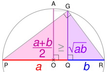
The altitude of a right triangle from its right angle to its hypotenuse is the geometric mean of the lengths of the segments the hypotenuse is split into. Using Pythagoras' theorem on the 3 triangles of sides (p+q, r, s), (r, p, h) and (s, h, q),
In the case of a right triangle, its altitude is the length of a line extending perpendicularly from the hypotenuse to its 90° vertex. Imagining that this line splits the hypotenuse into two segments, the geometric mean of these segment lengths is the length of the altitude. This property is known as the geometric mean theorem.
In an ellipse, the semi-minor axis is the geometric mean of the maximum and minimum distances of the ellipse from a focus; it is also the geometric mean of the semi-major axis and the semi-latus rectum. The semi-major axis of an ellipse is the geometric mean of the distance from the center to either focus and the distance from the center to either directrix.
Another way to think about it is as follows:
Consider a circle with radius . Now take two diametrically opposite points on the circle and apply pressure from both ends to deform it into an ellipse with semi-major and semi-minor axes of lengths and .
Since the area of the circle and the ellipse stays the same, we have:
The radius of the circle is the geometric mean of the semi-major and the semi-minor axes of the ellipse formed by deforming the circle.
Distance to the horizon of a sphere (ignoring the effect of atmospheric refraction when atmosphere is present) is equal to the geometric mean of the distance to the closest point of the sphere and the distance to the farthest point of the sphere.
The geometric mean is used in both in the approximation of squaring the circle by S.A. Ramanujan[11] and in the construction of the heptadecagon with "mean proportionals".[12]
Aspect ratios
Equal area comparison of the aspect ratios used by Kerns Powers to derive the SMPTE16:9 standard. TV 4:3/1.33 in red, 1.66 in orange, 16:9/1.77 in blue, 1.85 in yellow, Panavision/2.2 in mauve and CinemaScope/2.35 in purple.
The geometric mean has been used in choosing a compromise aspect ratio in film and video: given two aspect ratios, the geometric mean of them provides a compromise between them, distorting or cropping both in some sense equally. Concretely, two equal area rectangles (with the same center and parallel sides) of different aspect ratios intersect in a rectangle whose aspect ratio is the geometric mean, and their hull (smallest rectangle which contains both of them) likewise has the aspect ratio of their geometric mean.
In the choice of 16:9 aspect ratio by the SMPTE, balancing 2.35 and 4:3, the geometric mean is , and thus ... was chosen. This was discovered empirically by Kerns Powers, who cut out rectangles with equal areas and shaped them to match each of the popular aspect ratios. When overlapped with their center points aligned, he found that all of those aspect ratio rectangles fit within an outer rectangle with an aspect ratio of 1.77:1 and all of them also covered a smaller common inner rectangle with the same aspect ratio 1.77:1.[13] The value found by Powers is exactly the geometric mean of the extreme aspect ratios, 4:3(1.33:1) and CinemaScope(2.35:1), which is coincidentally close to (). The intermediate ratios have no effect on the result, only the two extreme ratios.
Applying the same geometric mean technique to 16:9 and 4:3 approximately yields the 14:9 (...) aspect ratio, which is likewise used as a compromise between these ratios.[14] In this case 14:9 is exactly the arithmetic mean of and , since 14 is the average of 16 and 12, while the precise geometric mean is but the two different means, arithmetic and geometric, are approximately equal because both numbers are sufficiently close to each other (a difference of less than 2%).
Paper formats
The geometric mean is also used to calculate B and C series paper formats. The format has an area which is the geometric mean of the areas of and . For example, the area of a B1 paper is , because it is the geometric mean of the areas of an A0 () and an A1 () paper ().
The same principle applies with the C series, whose area is the geometric mean of the A and B series. For example, the C4 format has an area which is the geometric mean of the areas of A4 and B4.
An advantage that comes from this relationship is that an A4 paper fits inside a C4 envelope, and both fit inside a B4 envelope.
Other applications
Spectral flatness: in signal processing, spectral flatness, a measure of how flat or spiky a spectrum is, is defined as the ratio of the geometric mean of the power spectrum to its arithmetic mean.
Anti-reflective coatings: In optical coatings, where reflection needs to be minimised between two media of refractive indices n0 and n2, the optimum refractive index n1 of the anti-reflective coating is given by the geometric mean: .
Labor compensation: The geometric mean of a subsistence wage and market value of the labor using capital of employer was suggested as the natural wage by Johann von Thünen in 1875.[16]
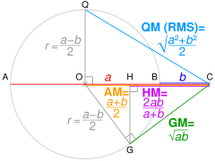
↑ If AC = a and BC = b. OC = AM of a and b, and radius r = QO = OG. Using Pythagoras' theorem, QC² = QO² + OC²∴ QC = √QO² + OC² = QM. Using Pythagoras' theorem, OC² = OG² + GC²∴ GC = √OC²− OG² = GM. Using similar triangles, HC/GC = GC/OC∴ HC = GC²/OC = HM.
Related Research Articles
In mathematics and statistics, the arithmetic mean, arithmetic average, or just the mean or average is the sum of a collection of numbers divided by the count of numbers in the collection. The collection is often a set of results from an experiment, an observational study, or a survey. The term "arithmetic mean" is preferred in some mathematics and statistics contexts because it helps distinguish it from other types of means, such as geometric and harmonic.
The number e is a mathematical constant approximately equal to 2.71828 that can be characterized in many ways. It is the base of the natural logarithm function. It is the limit of as n tends to infinity, an expression that arises in the computation of compound interest. It is the value at 1 of the (natural) exponential function, commonly denoted It is also the sum of the infinite series There are various other characterizations; see § Definitions and § Representations.
In mathematics, generalized means are a family of functions for aggregating sets of numbers. These include as special cases the Pythagorean means.
In mathematics, the harmonic mean is one of several kinds of average, and in particular, one of the Pythagorean means. It is sometimes appropriate for situations when the average rate is desired.
In mathematics, the logarithm to baseb is the inverse function of exponentiation with base b. That means that the logarithm of a number x to the baseb is the exponent to which b must be raised to produce x. For example, since 1000 = 103, the logarithm base of 1000 is 3, or log10 (1000) = 3. The logarithm of x to baseb is denoted as logb (x), or without parentheses, logbx. When the base is clear from the context or is irrelevant it is sometimes written log x.
A mean is a numeric quantity representing the center of a collection of numbers and is intermediate to the extreme values of a set of numbers. There are several kinds of means in mathematics, especially in statistics. Each attempts to summarize or typify a given group of data, illustrating the magnitude and sign of the data set. Which of these measures is most illuminating depends on what is being measured, and on context and purpose.
In probability theory and statistics, a normal distribution or Gaussian distribution is a type of continuous probability distribution for a real-valued random variable. The general form of its probability density function is The parameter is the mean or expectation of the distribution, while the parameter is the variance. The standard deviation of the distribution is . A random variable with a Gaussian distribution is said to be normally distributed, and is called a normal deviate.
The natural logarithm of a number is its logarithm to the base of the mathematical constant e, which is an irrational and transcendental number approximately equal to 2.718281828459. The natural logarithm of x is generally written as ln x, logex, or sometimes, if the base e is implicit, simply log x. Parentheses are sometimes added for clarity, giving ln(x), loge(x), or log(x). This is done particularly when the argument to the logarithm is not a single symbol, so as to prevent ambiguity.
In mathematics, a square root of a number x is a number y such that ; in other words, a number y whose square is x. For example, 4 and −4 are square roots of 16 because .
The imaginary unit or unit imaginary number is a solution to the quadratic equation x2 + 1 = 0. Although there is no real number with this property, i can be used to extend the real numbers to what are called complex numbers, using addition and multiplication. A simple example of the use of i in a complex number is 2 + 3i.
In probability theory, a log-normal (or lognormal) distribution is a continuous probability distribution of a random variable whose logarithm is normally distributed. Thus, if the random variable X is log-normally distributed, then Y = ln(X) has a normal distribution. Equivalently, if Y has a normal distribution, then the exponential function of Y, X = exp(Y), has a log-normal distribution. A random variable which is log-normally distributed takes only positive real values. It is a convenient and useful model for measurements in exact and engineering sciences, as well as medicine, economics and other topics (e.g., energies, concentrations, lengths, prices of financial instruments, and other metrics).
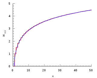
In mathematics, the n-th harmonic number is the sum of the reciprocals of the first n natural numbers:
In probability theory and statistics, the geometric standard deviation (GSD) describes how spread out are a set of numbers whose preferred average is the geometric mean. For such data, it may be preferred to the more usual standard deviation. Note that unlike the usual arithmetic standard deviation, the geometric standard deviation is a multiplicative factor, and thus is dimensionless, rather than having the same dimension as the input values. Thus, the geometric standard deviation may be more appropriately called geometric SD factor. When using geometric SD factor in conjunction with geometric mean, it should be described as "the range from to, and one cannot add/subtract "geometric SD factor" to/from geometric mean.
In mathematics, the inequality of arithmetic and geometric means, or more briefly the AM–GM inequality, states that the arithmetic mean of a list of non-negative real numbers is greater than or equal to the geometric mean of the same list; and further, that the two means are equal if and only if every number in the list is the same.
A mathematical coincidence is said to occur when two expressions with no direct relationship show a near-equality which has no apparent theoretical explanation.
In mathematics, the three classical Pythagorean means are the arithmetic mean (AM), the geometric mean (GM), and the harmonic mean (HM). These means were studied with proportions by Pythagoreans and later generations of Greek mathematicians because of their importance in geometry and music.
In mathematics, the logarithmic mean is a function of two non-negative numbers which is equal to their difference divided by the logarithm of their quotient. This calculation is applicable in engineering problems involving heat and mass transfer.
In mathematics, a contraharmonic mean is a function complementary to the harmonic mean. The contraharmonic mean is a special case of the Lehmer mean, , where p = 2.
A geometric progression, also known as a geometric sequence, is a mathematical sequence of non-zero numbers where each term after the first is found by multiplying the previous one by a fixed, non-zero number called the common ratio. For example, the sequence 2, 6, 18, 54, ... is a geometric progression with common ratio 3. Similarly 10, 5, 2.5, 1.25, ... is a geometric sequence with common ratio 1/2.
This page is based on this Wikipedia article Text is available under the CC BY-SA 4.0 license; additional terms may apply. Images, videos and audio are available under their respective licenses.
![Example of the geometric mean:
l
g
{\displaystyle l_{g}}
(red) is the geometric mean of
l
1
{\displaystyle l_{1}}
and
l
2
{\displaystyle l_{2}}
, is an example in which the line segment
l
2
(
B
C
-
)
{\displaystyle l_{2}\;({\overline {BC}})}
is given as a perpendicular to
A
B
-
{\displaystyle {\overline {AB}}}
.
A
C
-
{\displaystyle {\overline {AC}}}
is the diameter of a circle and
B
C
-
[?]
B
C
'
-
{\displaystyle {\overline {BC}}\cong {\overline {BC'}}}
. (Note: 10-second pause between each animation run). 01-Mittlere Proportionale.gif](http://upload.wikimedia.org/wikipedia/commons/thumb/f/fa/01-Mittlere_Proportionale.gif/400px-01-Mittlere_Proportionale.gif)


![The altitude of a right triangle from its right angle to its hypotenuse is the geometric mean of the lengths of the segments the hypotenuse is split into. Using Pythagoras' theorem on the 3 triangles of sides (p + q, r, s ), (r, p, h ) and (s, h, q ),
(
p
+
q
)
2
=
r
2
+
s
2
p
2
+
2
p
q
+
q
2
=
p
2
+
h
2
[?]
+
h
2
+
q
2
[?]
2
p
q
=
2
h
2
[?]
h
=
p
q
{\displaystyle {\begin{aligned}(p+q)^{2}\;\;&=\quad r^{2}\;\;\,+\quad s^{2}\\p^{2}\!\!+\!2pq\!+\!q^{2}&=\overbrace {p^{2}\!\!+\!h^{2}} +\overbrace {h^{2}\!\!+\!q^{2}} \\2pq\quad \;\;\;&=2h^{2}\;\therefore h\!=\!{\sqrt {pq}}\\\end{aligned}}} Right angle altitude.svg](http://upload.wikimedia.org/wikipedia/commons/thumb/c/cf/Right_angle_altitude.svg/220px-Right_angle_altitude.svg.png)