Percentile

In statistics, a k-thpercentile, also known as percentile score or centile, is a score below which a given percentage k of scores in its frequency distribution falls ("exclusive" definition) or a score at or below which a given percentage falls ("inclusive" definition). Percentiles are expressed in the same unit of measurement as the input scores, not in percent; for example, if the scores refer to human weight, the corresponding percentiles will be expressed in kilograms or pounds. In the limit of an infinite sample size, the percentile approximates the percentile function , the inverse of the cumulative distribution function.

Percentiles are a type of quantiles, obtained adopting a subdivision into 100 groups. The 25th percentile is also known as the first quartile (Q₁), the 50th percentile as the median or second quartile (Q₂), and the 75th percentile as the third quartile (Q₃). For example, the 50th percentile (median) is the score below (or at or below, depending on the definition) which 50% of the scores in the distribution are found.

A related quantity is the percentile rank of a score, expressed in percent, which represents the fraction of scores in its distribution that are less than it, an exclusive definition. Percentile scores and percentile ranks are often used in the reporting of test scores from norm-referenced tests, but, as just noted, they are not the same. For percentile ranks, a score is given and a percentage is computed. Percentile ranks are exclusive: if the percentile rank for a specified score is 90%, then 90% of the scores were lower. In contrast, for percentiles a percentage is given and a corresponding score is determined, which can be either exclusive or inclusive. The score for a specified percentage (e.g., 90th) indicates a score below which (exclusive definition) or at or below which (inclusive definition) other scores in the distribution fall.

Definitions

There is no standard definition of percentile, ^{[1] [2] [3]} however all definitions yield similar results when the number of observations is very large and the probability distribution is continuous. ^[4] In the limit, as the sample size approaches infinity, the 100p^th percentile (0<p<1) approximates the inverse of the cumulative distribution function (CDF) thus formed, evaluated at p, as p approximates the CDF. This can be seen as a consequence of the Glivenko–Cantelli theorem. Some methods for calculating the percentiles are given below.

The normal distribution and percentiles

Representation of the three-sigma rule. The dark blue zone represents observations within one standard deviation (σ) to either side of the mean (μ), which accounts for about 68.3% of the population. Two standard deviations from the mean (dark and medium blue) account for about 95.4%, and three standard deviations (dark, medium, and light blue) for about 99.7%.

The methods given in the calculation methods section (below) are approximations for use in small-sample statistics. In general terms, for very large populations following a normal distribution, percentiles may often be represented by reference to a normal curve plot. The normal distribution is plotted along an axis scaled to standard deviations, or sigma (${\displaystyle \sigma }$) units. Mathematically, the normal distribution extends to negative infinity on the left and positive infinity on the right. Note, however, that only a very small proportion of individuals in a population will fall outside the −3σ to +3σ range. For example, with human heights very few people are above the +3σ height level.

Percentiles represent the area under the normal curve, increasing from left to right. Each standard deviation represents a fixed percentile. Thus, rounding to two decimal places, −3σ is the 0.13th percentile, −2σ the 2.28th percentile, −1σ the 15.87th percentile, 0σ the 50th percentile (both the mean and median of the distribution), +1σ the 84.13th percentile, +2σ the 97.72nd percentile, and +3σ the 99.87th percentile. This is related to the 68–95–99.7 rule or the three-sigma rule. Note that in theory the 0th percentile falls at negative infinity and the 100th percentile at positive infinity, although in many practical applications, such as test results, natural lower and/or upper limits are enforced.

Applications

When ISPs bill "burstable" internet bandwidth, the 95th or 98th percentile usually cuts off the top 5% or 2% of bandwidth peaks in each month, and then bills at the nearest rate. In this way, infrequent peaks are ignored, and the customer is charged in a fairer way. The reason this statistic is so useful in measuring data throughput is that it gives a very accurate picture of the cost of the bandwidth. The 95th percentile says that 95% of the time, the usage is below this amount: so, the remaining 5% of the time, the usage is above that amount.

Physicians will often use infant and children's weight and height to assess their growth in comparison to national averages and percentiles which are found in growth charts.

The 85th percentile speed of traffic on a road is often used as a guideline in setting speed limits and assessing whether such a limit is too high or low. ^{[5] [6]}

In finance, value at risk is a standard measure to assess (in a model-dependent way) the quantity under which the value of the portfolio is not expected to sink within a given period of time and given a confidence value.

Calculation methods

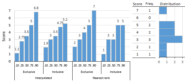
Interpolated and nearest-rank, exclusive and inclusive, percentiles for 10-score distribution

Interpolated and nearest-rank, exclusive and inclusive, percentiles for 10-score distribution

There are many formulas or algorithms ^[7] for a percentile score. Hyndman and Fan ^[1] identified nine and most statistical and spreadsheet software use one of the methods they describe. ^[8] Algorithms either return the value of a score that exists in the set of scores (nearest-rank methods) or interpolate between existing scores and are either exclusive or inclusive.

Nearest-rank methods (exclusive/inclusive)

PC: percentile specified	0.10	0.25	0.50	0.75	0.90
N: Number of scores	10	10	10	10	10
OR: ordinal rank = PC × N	1	2.5	5	7.5	9
Rank: >OR / ≥OR	2/1	3/3	6/5	8/8	10/9
Score at rank (exc/inc)	2/1	3/3	4/3	5/5	7/5

The figure shows a 10-score distribution, illustrates the percentile scores that result from these different algorithms, and serves as an introduction to the examples given subsequently. The simplest are nearest-rank methods that return a score from the distribution, although compared to interpolation methods, results can be a bit crude. The Nearest-Rank Methods table shows the computational steps for exclusive and inclusive methods.

Interpolated methods (exclusive/inclusive)

PC: percentile specified	0.10	0.25	0.50	0.75	0.90
N: number of scores	10	10	10	10	10
OR: PC×(N+1) / PC×(N−1)+1	1.1/1.9	2.75/3.25	5.5/5.5	8.25/7.75	9.9/9.1
LoRank: OR truncated	1/1	2/3	5/5	8/7	9/9
HIRank: OR rounded up	2/2	3/4	6/6	9/8	10/10
LoScore: score at LoRank	1/1	2/3	3/3	5/4	5/5
HiScore: score at HiRank	2/2	3/3	4/4	5/5	7/7
Difference: HiScore − LoScore	1/1	1/0	1/1	0/1	2/2
Mod: fractional part of OR	0.1/0.9	0.75/0.25	0.5/0.5	0.25/0.75	0.9/0.1
Interpolated score (exc/inc) = LoScore + Mod × Difference	1.1/1.9	2.75/3	3.5/3.5	5/4.75	6.8/5.2

Interpolation methods, as the name implies, can return a score that is between scores in the distribution. Algorithms used by statistical programs typically use interpolation methods, for example, the percentile.exc and percentile.inc functions in Microsoft Excel. The Interpolated Methods table shows the computational steps.

The nearest-rank method

The percentile values for the ordered list {15, 20, 35, 40, 50}

One definition of percentile, often given in texts, is that the P-th percentile ${\displaystyle (0<P\leq 100)}$ of a list of N ordered values (sorted from least to greatest) is the smallest value in the list such that no more than P percent of the data is strictly less than the value and at least P percent of the data is less than or equal to that value. This is obtained by first calculating the ordinal rank and then taking the value from the ordered list that corresponds to that rank. The ordinal rank n is calculated using this formula

${\displaystyle n=\left\lceil {\frac {P}{100}}\times N\right\rceil .}$

• Using the nearest-rank method on lists with fewer than 100 distinct values can result in the same value being used for more than one percentile.
• A percentile calculated using the nearest-rank method will always be a member of the original ordered list.
• The 100th percentile is defined to be the largest value in the ordered list.

The linear interpolation between closest ranks method

An alternative to rounding used in many applications is to use linear interpolation between adjacent ranks.

All of the following variants have the following in common. Given the order statistics

${\displaystyle \{v_{i},i=1,2,\ldots ,N:v_{i+1}\geq v_{i},\forall i=1,2,\ldots ,N-1\},}$

we seek a linear interpolation function that passes through the points ${\displaystyle (v_{i},i)}$. This is simply accomplished by

${\displaystyle v(x)=v_{\lfloor x\rfloor }+(x{\bmod {1}})(v_{\lfloor x\rfloor +1}-v_{\lfloor x\rfloor }),\forall x\in [1,N]:v(i)=v_{i}{\text{, for }}i=1,2,\ldots ,N,}$

where ${\displaystyle \lfloor x\rfloor }$ uses the floor function to represent the integral part of positive x, whereas ${\displaystyle x{\bmod {1}}}$ uses the mod function to represent its fractional part (the remainder after division by 1). (Note that, though at the endpoint ${\displaystyle x=N}$, ${\displaystyle v_{\lfloor x\rfloor +1}}$ is undefined, it does not need to be because it is multiplied by ${\displaystyle x{\bmod {1}}=0}$.) As we can see, x is the continuous version of the subscript i, linearly interpolating v between adjacent nodes.

There are two ways in which the variant approaches differ. The first is in the linear relationship between the rankx, the percent rank${\displaystyle P=100p}$, and a constant that is a function of the sample size N:

${\displaystyle x=f(p,N)=(N+c_{1})p+c_{2}.}$

There is the additional requirement that the midpoint of the range ${\displaystyle (1,N)}$, corresponding to the median, occur at ${\displaystyle p=0.5}$:

${\displaystyle {\begin{aligned}f(0.5,N)&={\frac {N+c_{1}}{2}}+c_{2}={\frac {N+1}{2}}\\\therefore 2c_{2}+c_{1}&=1\end{aligned}},}$

and our revised function now has just one degree of freedom, looking like this:

${\displaystyle x=f(p,N)=(N+1-2C)p+C.}$

The second way in which the variants differ is in the definition of the function near the margins of the ${\displaystyle [0,1]}$ range of p: ${\displaystyle f(p,N)}$ should produce, or be forced to produce, a result in the range ${\displaystyle [1,N]}$, which may mean the absence of a one-to-one correspondence in the wider region. One author has suggested a choice of ${\displaystyle C={\tfrac {1}{2}}(1+\xi )}$ where ξ is the shape of the Generalized extreme value distribution which is the extreme value limit of the sampled distribution.

First variant, C = 1/2

The result of using each of the three variants on the ordered list {15, 20, 35, 40, 50}

(Sources: Matlab "prctile" function, ^{[9] [10]} )

${\displaystyle x=f(p)={\begin{cases}Np+{\frac {1}{2}},\forall p\in \left[p_{1},p_{N}\right],\\1,\forall p\in \left[0,p_{1}\right],\\N,\forall p\in \left[p_{N},1\right].\end{cases}}}$

where

${\displaystyle p_{i}={\frac {1}{N}}\left(i-{\frac {1}{2}}\right),i\in [1,N]\cap \mathbb {N} }$

${\displaystyle \therefore p_{1}={\frac {1}{2N}},p_{N}={\frac {2N-1}{2N}}.}$

Furthermore, let

${\displaystyle P_{i}=100p_{i}.}$

The inverse relationship is restricted to a narrower region:

${\displaystyle p={\frac {1}{N}}\left(x-{\frac {1}{2}}\right),x\in (1,N)\cap \mathbb {R} .}$

Second variant, C = 1

(Source: Some software packages, including NumPy ^[11] and Microsoft Excel ^[3] (up to and including version 2013 by means of the PERCENTILE.INC function). Noted as an alternative by NIST ^[8] )

${\displaystyle x=f(p,N)=p(N-1)+1{\text{, }}p\in [0,1]}$

${\displaystyle \therefore p={\frac {x-1}{N-1}}{\text{, }}x\in [1,N].}$

Note that the ${\displaystyle x\leftrightarrow p}$ relationship is one-to-one for ${\displaystyle p\in [0,1]}$, the only one of the three variants with this property; hence the "INC" suffix, for inclusive, on the Excel function.

Third variant, C = 0

(The primary variant recommended by NIST. ^[8] Adopted by Microsoft Excel since 2010 by means of PERCENTIL.EXC function. However, as the "EXC" suffix indicates, the Excel version excludes both endpoints of the range of p, i.e., ${\displaystyle p\in (0,1)}$, whereas the "INC" version, the second variant, does not; in fact, any number smaller than ${\displaystyle {\frac {1}{N+1}}}$ is also excluded and would cause an error.)

${\displaystyle x=f(p,N)={\begin{cases}1{\text{, }}p\in \left[0,{\frac {1}{N+1}}\right]\\p(N+1){\text{, }}p\in \left({\frac {1}{N+1}},{\frac {N}{N+1}}\right)\\N{\text{, }}p\in \left[{\frac {N}{N+1}},1\right]\end{cases}}.}$

The inverse is restricted to a narrower region:

${\displaystyle p={\frac {x}{N+1}}{\text{, }}x\in (0,N).}$

The weighted percentile method

See also: Weighted median

In addition to the percentile function, there is also a weighted percentile, where the percentage in the total weight is counted instead of the total number. There is no standard function for a weighted percentile. One method extends the above approach in a natural way.

Suppose we have positive weights ${\displaystyle w_{1},w_{2},w_{3},\dots ,w_{N}}$ associated, respectively, with our N sorted sample values. Let

${\displaystyle S_{N}=\sum _{k=1}^{N}w_{k},}$

the sum of the weights. Then the formulas above are generalized by taking

${\displaystyle p_{n}={\frac {1}{S_{N}}}\left(S_{n}-{\frac {w_{n}}{2}}\right)}$ when ${\displaystyle C=1/2}$,

or

${\displaystyle p_{n}={\frac {S_{n}-Cw_{n}}{S_{N}+(1-2C)w_{n}}}}$ for general ${\displaystyle C}$,

and

${\displaystyle v=v_{k}+{\frac {P-p_{k}}{p_{k+1}-p_{k}}}(v_{k+1}-v_{k}).}$

The 50% weighted percentile is known as the weighted median.

See also

• Mathematics portal

• Decile
• Percentile rank
• Quantile
• Summary statistics

References

1. Hyndman, Rob J.; Fan, Yanan (November 1996). "Sample Quantiles in Statistical Packages". American Statistician. American Statistical Association. 50 (4): 361–365. doi:10.2307/2684934. JSTOR   2684934.
2. Lane, David. "Percentiles" . Retrieved 2007-09-15.
3. Pottel, Hans. "Statistical flaws in Excel" (PDF). Archived from the original (PDF) on 2013-06-04. Retrieved 2013-03-25.
4. Schoonjans F, De Bacquer D, Schmid P (2011). "Estimation of population percentiles". Epidemiology. 22 (5): 750–751. doi:10.1097/EDE.0b013e318225c1de. PMC   3171208 . PMID   21811118.
5. Johnson, Robert; Kuby, Patricia (2007), "Applied Example 2.15, The 85th Percentile Speed Limit: Going With 85% of the Flow", Elementary Statistics (10th ed.), Cengage Learning, p. 102, ISBN   9781111802493 .
6. "Rational Speed Limits and the 85th Percentile Speed" (PDF). lsp.org. Louisiana State Police. Archived from the original (PDF) on 23 September 2018. Retrieved 28 October 2018.
7. Wessa, P (2021). "Percentiles in Free Statistics Software". Office for Research Development and Education. Retrieved 13 November 2021.
8. "Engineering Statistics Handbook: Percentile". NIST . Retrieved 2009-02-18.
9. "Matlab Statistics Toolbox – Percentiles" . Retrieved 2006-09-15., This is equivalent to Method 5 discussed here
10. Langford, E. (2006). "Quartiles in Elementary Statistics". Journal of Statistics Education. 14 (3). doi: 10.1080/10691898.2006.11910589 .
11. "NumPy 1.12 documentation". SciPy . Retrieved 2017-03-19.