Cumulative distribution function

Cumulative distribution function for the exponential distribution

Cumulative distribution function for the normal distribution

In probability theory and statistics, the cumulative distribution function (CDF) of a real-valued random variable ${\displaystyle X}$, or just distribution function of ${\displaystyle X}$, evaluated at ${\displaystyle x}$, is the probability that ${\displaystyle X}$ will take a value less than or equal to ${\displaystyle x}$. ^[1]

Every probability distribution supported on the real numbers, discrete or "mixed" as well as continuous, is uniquely identified by a right-continuous monotone increasing function (a càdlàg function) ${\displaystyle F\colon \mathbb {R} \rightarrow [0,1]}$ satisfying ${\displaystyle \lim _{x\rightarrow -\infty }F(x)=0}$ and ${\displaystyle \lim _{x\rightarrow \infty }F(x)=1}$.

In the case of a scalar continuous distribution, it gives the area under the probability density function from negative infinity to ${\displaystyle x}$. Cumulative distribution functions are also used to specify the distribution of multivariate random variables.

Definition

The cumulative distribution function of a real-valued random variable ${\displaystyle X}$ is the function given by ^{[2] : p. 77}

$${\displaystyle F_{X}(x)=\operatorname {P} (X\leq x)}$$

(Eq.1)

where the right-hand side represents the probability that the random variable ${\displaystyle X}$ takes on a value less than or equal to ${\displaystyle x}$.

The probability that ${\displaystyle X}$ lies in the semi-closed interval ${\displaystyle (a,b]}$, where ${\displaystyle a<b}$, is therefore ^{[2] : p. 84}

$${\displaystyle \operatorname {P} (a<X\leq b)=F_{X}(b)-F_{X}(a)}$$

(Eq.2)

In the definition above, the "less than or equal to" sign, "≤", is a convention, not a universally used one (e.g. Hungarian literature uses "<"), but the distinction is important for discrete distributions. The proper use of tables of the binomial and Poisson distributions depends upon this convention. Moreover, important formulas like Paul Lévy's inversion formula for the characteristic function also rely on the "less than or equal" formulation.

If treating several random variables ${\displaystyle X,Y,\ldots }$ etc. the corresponding letters are used as subscripts while, if treating only one, the subscript is usually omitted. It is conventional to use a capital ${\displaystyle F}$ for a cumulative distribution function, in contrast to the lower-case ${\displaystyle f}$ used for probability density functions and probability mass functions. This applies when discussing general distributions: some specific distributions have their own conventional notation, for example the normal distribution uses ${\displaystyle \Phi }$ and ${\displaystyle \phi }$ instead of ${\displaystyle F}$ and ${\displaystyle f}$, respectively.

The probability density function of a continuous random variable can be determined from the cumulative distribution function by differentiating ^[3] using the Fundamental Theorem of Calculus; i.e. given ${\displaystyle F(x)}$,

$${\displaystyle f(x)={\frac {dF(x)}{dx}}}$$

as long as the derivative exists.

The CDF of a continuous random variable ${\displaystyle X}$ can be expressed as the integral of its probability density function ${\displaystyle f_{X}}$ as follows: ^{[2] : p. 86}

$${\displaystyle F_{X}(x)=\int _{-\infty }^{x}f_{X}(t)\,dt.}$$

In the case of a random variable ${\displaystyle X}$ which has distribution having a discrete component at a value ${\displaystyle b}$,

$${\displaystyle \operatorname {P} (X=b)=F_{X}(b)-\lim _{x\to b^{-}}F_{X}(x).}$$

If ${\displaystyle F_{X}}$ is continuous at ${\displaystyle b}$, this equals zero and there is no discrete component at ${\displaystyle b}$.

Properties

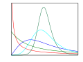
From top to bottom, the cumulative distribution function of a discrete probability distribution, continuous probability distribution, and a distribution which has both a continuous part and a discrete part.

Example of a cumulative distribution function with a countably infinite set of discontinuities.

Every cumulative distribution function ${\displaystyle F_{X}}$ is non-decreasing ^{[2] : p. 78} and right-continuous, ^{[2] : p. 79} which makes it a càdlàg function. Furthermore,

$${\displaystyle \lim _{x\to -\infty }F_{X}(x)=0,\quad \lim _{x\to +\infty }F_{X}(x)=1.}$$

Every function with these four properties is a CDF, i.e., for every such function, a random variable can be defined such that the function is the cumulative distribution function of that random variable.

If ${\displaystyle X}$ is a purely discrete random variable, then it attains values ${\displaystyle x_{1},x_{2},\ldots }$ with probability ${\displaystyle p_{i}=p(x_{i})}$, and the CDF of ${\displaystyle X}$ will be discontinuous at the points ${\displaystyle x_{i}}$:

$${\displaystyle F_{X}(x)=\operatorname {P} (X\leq x)=\sum _{x_{i}\leq x}\operatorname {P} (X=x_{i})=\sum _{x_{i}\leq x}p(x_{i}).}$$

If the CDF ${\displaystyle F_{X}}$ of a real valued random variable ${\displaystyle X}$ is continuous, then ${\displaystyle X}$ is a continuous random variable; if furthermore ${\displaystyle F_{X}}$ is absolutely continuous, then there exists a Lebesgue-integrable function ${\displaystyle f_{X}(x)}$ such that

$${\displaystyle F_{X}(b)-F_{X}(a)=\operatorname {P} (a<X\leq b)=\int _{a}^{b}f_{X}(x)\,dx}$$

for all real numbers ${\displaystyle a}$ and ${\displaystyle b}$. The function ${\displaystyle f_{X}}$ is equal to the derivative of ${\displaystyle F_{X}}$ almost everywhere, and it is called the probability density function of the distribution of ${\displaystyle X}$.

If ${\displaystyle X}$ has finite L1-norm, that is, the expectation of ${\displaystyle |X|}$ is finite, then the expectation is given by the Riemann–Stieltjes integral

$${\displaystyle \mathbb {E} [X]=\int _{-\infty }^{\infty }tdF_{X}(t)}$$

and for any ${\displaystyle x\geq 0}$,

CDF plot with two red rectangles, illustrating ${\displaystyle x(1-F_{X}(x))\leq \int _{x}^{\infty }tdF_{X}(t)}$ and ${\displaystyle xF_{X}(-x)\leq \int _{-\infty }^{-x}(-t)dF_{X}(t)}$.

$${\displaystyle {\begin{aligned}x(1-F_{X}(x))&\leq \int _{x}^{\infty }tdF_{X}(t)\\xF_{X}(-x)&\leq \int _{-\infty }^{-x}(-t)dF_{X}(t)\end{aligned}}}$$

as shown in the diagram. In particular, we have

$${\displaystyle \lim _{x\to -\infty }xF(x)=0,\quad \lim _{x\to +\infty }x(1-F(x))=0.}$$

Examples

As an example, suppose ${\displaystyle X}$ is uniformly distributed on the unit interval ${\displaystyle [0,1]}$.

Then the CDF of ${\displaystyle X}$ is given by

$${\displaystyle F_{X}(x)={\begin{cases}0&:\ x<0\\x&:\ 0\leq x\leq 1\\1&:\ x>1\end{cases}}}$$

Suppose instead that ${\displaystyle X}$ takes only the discrete values 0 and 1, with equal probability.

Then the CDF of ${\displaystyle X}$ is given by

$${\displaystyle F_{X}(x)={\begin{cases}0&:\ x<0\\1/2&:\ 0\leq x<1\\1&:\ x\geq 1\end{cases}}}$$

Suppose ${\displaystyle X}$ is exponential distributed. Then the CDF of ${\displaystyle X}$ is given by

$${\displaystyle F_{X}(x;\lambda )={\begin{cases}1-e^{-\lambda x}&x\geq 0,\\0&x<0.\end{cases}}}$$

Here λ > 0 is the parameter of the distribution, often called the rate parameter.

Suppose ${\displaystyle X}$ is normal distributed. Then the CDF of ${\displaystyle X}$ is given by

$${\displaystyle F(x;\mu ,\sigma )={\frac {1}{\sigma {\sqrt {2\pi }}}}\int _{-\infty }^{x}\exp \left(-{\frac {(t-\mu )^{2}}{2\sigma ^{2}}}\right)\,dt.}$$

Here the parameter ${\displaystyle \mu }$ is the mean or expectation of the distribution; and ${\displaystyle \sigma }$ is its standard deviation.

A table of the CDF of the standard normal distribution is often used in statistical applications, where it is named the standard normal table, the unit normal table, or the Z table.

Suppose ${\displaystyle X}$ is binomial distributed. Then the CDF of ${\displaystyle X}$ is given by

$${\displaystyle F(k;n,p)=\Pr(X\leq k)=\sum _{i=0}^{\lfloor k\rfloor }{n \choose i}p^{i}(1-p)^{n-i}}$$

Here ${\displaystyle p}$ is the probability of success and the function denotes the discrete probability distribution of the number of successes in a sequence of ${\displaystyle n}$ independent experiments, and ${\displaystyle \lfloor k\rfloor }$ is the "floor" under ${\displaystyle k}$, i.e. the greatest integer less than or equal to ${\displaystyle k}$.

Derived functions

Complementary cumulative distribution function (tail distribution)

Sometimes, it is useful to study the opposite question and ask how often the random variable is above a particular level. This is called the complementary cumulative distribution function (ccdf) or simply the tail distribution or exceedance, and is defined as

$${\displaystyle {\bar {F}}_{X}(x)=\operatorname {P} (X>x)=1-F_{X}(x).}$$

This has applications in statistical hypothesis testing, for example, because the one-sided p-value is the probability of observing a test statistic at least as extreme as the one observed. Thus, provided that the test statistic, T, has a continuous distribution, the one-sided p-value is simply given by the ccdf: for an observed value ${\displaystyle t}$ of the test statistic

$${\displaystyle p=\operatorname {P} (T\geq t)=\operatorname {P} (T>t)=1-F_{T}(t).}$$

In survival analysis, ${\displaystyle {\bar {F}}_{X}(x)}$ is called the survival function and denoted ${\displaystyle S(x)}$, while the term reliability function is common in engineering.

Properties

• For a non-negative continuous random variable having an expectation, Markov's inequality states that ^[4]
  $${\displaystyle {\bar {F}}_{X}(x)\leq {\frac {\operatorname {E} (X)}{x}}.}$$
• As ${\displaystyle x\to \infty ,{\bar {F}}_{X}(x)\to 0}$, and in fact ${\displaystyle {\bar {F}}_{X}(x)=o(1/x)}$ provided that ${\displaystyle \operatorname {E} (X)}$ is finite.
  Proof:^{[ citation needed ]}
  Assuming ${\displaystyle X}$ has a density function ${\displaystyle f_{X}}$, for any ${\displaystyle c>0}$
  $${\displaystyle \operatorname {E} (X)=\int _{0}^{\infty }xf_{X}(x)\,dx\geq \int _{0}^{c}xf_{X}(x)\,dx+c\int _{c}^{\infty }f_{X}(x)\,dx}$$
  Then, on recognizing
  $${\displaystyle {\bar {F}}_{X}(c)=\int _{c}^{\infty }f_{X}(x)\,dx}$$
  and rearranging terms,
  $${\displaystyle 0\leq c{\bar {F}}_{X}(c)\leq \operatorname {E} (X)-\int _{0}^{c}xf_{X}(x)\,dx\to 0{\text{ as }}c\to \infty }$$
  as claimed.
• For a random variable having an expectation,
  $${\displaystyle \operatorname {E} (X)=\int _{0}^{\infty }{\bar {F}}_{X}(x)\,dx-\int _{-\infty }^{0}F_{X}(x)\,dx}$$
  and for a non-negative random variable the second term is 0.
  If the random variable can only take non-negative integer values, this is equivalent to
  $${\displaystyle \operatorname {E} (X)=\sum _{n=0}^{\infty }{\bar {F}}_{X}(n).}$$

Folded cumulative distribution

Example of the folded cumulative distribution for a normal distribution function with an expected value of 0 and a standard deviation of 1.

While the plot of a cumulative distribution ${\displaystyle F}$ often has an S-like shape, an alternative illustration is the folded cumulative distribution or mountain plot, which folds the top half of the graph over, ^{[5] [6]} that is

${\displaystyle F_{\text{fold}}(x)=F(x)1_{\{F(x)\leq 0.5\}}+(1-F(x))1_{\{F(x)>0.5\}}}$

where ${\displaystyle 1_{\{A\}}}$ denotes the indicator function and the second summand is the survivor function, thus using two scales, one for the upslope and another for the downslope. This form of illustration emphasises the median, dispersion (specifically, the mean absolute deviation from the median ^[7] ) and skewness of the distribution or of the empirical results.

Inverse distribution function (quantile function)

Main article: Quantile function

If the CDF F is strictly increasing and continuous then ${\displaystyle F^{-1}(p),p\in [0,1],}$ is the unique real number ${\displaystyle x}$ such that ${\displaystyle F(x)=p}$. This defines the inverse distribution function or quantile function.

Some distributions do not have a unique inverse (for example if ${\displaystyle f_{X}(x)=0}$ for all ${\displaystyle a<x<b}$, causing ${\displaystyle F_{X}}$ to be constant). In this case, one may use the generalized inverse distribution function, which is defined as

${\displaystyle F^{-1}(p)=\inf\{x\in \mathbb {R} :F(x)\geq p\},\quad \forall p\in [0,1].}$

• Example 1: The median is ${\displaystyle F^{-1}(0.5)}$.
• Example 2: Put ${\displaystyle \tau =F^{-1}(0.95)}$. Then we call ${\displaystyle \tau }$ the 95th percentile.

Some useful properties of the inverse cdf (which are also preserved in the definition of the generalized inverse distribution function) are:

1. ${\displaystyle F^{-1}}$ is nondecreasing ^[8]
2. ${\displaystyle F^{-1}(F(x))\leq x}$
3. ${\displaystyle F(F^{-1}(p))\geq p}$
4. ${\displaystyle F^{-1}(p)\leq x}$ if and only if ${\displaystyle p\leq F(x)}$
5. If ${\displaystyle Y}$ has a ${\displaystyle U[0,1]}$ distribution then ${\displaystyle F^{-1}(Y)}$ is distributed as ${\displaystyle F}$. This is used in random number generation using the inverse transform sampling-method.
6. If ${\displaystyle \{X_{\alpha }\}}$ is a collection of independent ${\displaystyle F}$-distributed random variables defined on the same sample space, then there exist random variables ${\displaystyle Y_{\alpha }}$ such that ${\displaystyle Y_{\alpha }}$ is distributed as ${\displaystyle U[0,1]}$ and ${\displaystyle F^{-1}(Y_{\alpha })=X_{\alpha }}$ with probability 1 for all ${\displaystyle \alpha }$.^{[ citation needed ]}

The inverse of the cdf can be used to translate results obtained for the uniform distribution to other distributions.

Empirical distribution function

The empirical distribution function is an estimate of the cumulative distribution function that generated the points in the sample. It converges with probability 1 to that underlying distribution. A number of results exist to quantify the rate of convergence of the empirical distribution function to the underlying cumulative distribution function. ^[9]

Multivariate case

Definition for two random variables

When dealing simultaneously with more than one random variable the joint cumulative distribution function can also be defined. For example, for a pair of random variables ${\displaystyle X,Y}$, the joint CDF ${\displaystyle F_{XY}}$ is given by ^{[2] : p. 89}

$${\displaystyle F_{X,Y}(x,y)=\operatorname {P} (X\leq x,Y\leq y)}$$

(Eq.3)

where the right-hand side represents the probability that the random variable ${\displaystyle X}$ takes on a value less than or equal to ${\displaystyle x}$and that ${\displaystyle Y}$ takes on a value less than or equal to ${\displaystyle y}$.

Example of joint cumulative distribution function:

For two continuous variables X and Y:

$${\displaystyle \Pr(a<X<b{\text{ and }}c<Y<d)=\int _{a}^{b}\int _{c}^{d}f(x,y)\,dy\,dx;}$$

For two discrete random variables, it is beneficial to generate a table of probabilities and address the cumulative probability for each potential range of X and Y, and here is the example: ^[10]

given the joint probability mass function in tabular form, determine the joint cumulative distribution function.

	Y = 2	Y = 4	Y = 6	Y = 8
X = 1	0	0.1	0	0.1
X = 3	0	0	0.2	0
X = 5	0.3	0	0	0.15
X = 7	0	0	0.15	0

Solution: using the given table of probabilities for each potential range of X and Y, the joint cumulative distribution function may be constructed in tabular form:

	Y < 2	Y ≤ 2	Y ≤ 4	Y ≤ 6	Y ≤ 8
X < 1	0	0	0	0	0
X ≤ 1	0	0	0.1	0.1	0.2
X ≤ 3	0	0	0.1	0.3	0.4
X ≤ 5	0	0.3	0.4	0.6	0.85
X ≤ 7	0	0.3	0.4	0.75	1

Definition for more than two random variables

For ${\displaystyle N}$ random variables ${\displaystyle X_{1},\ldots ,X_{N}}$, the joint CDF ${\displaystyle F_{X_{1},\ldots ,X_{N}}}$ is given by

$${\displaystyle F_{X_{1},\ldots ,X_{N}}(x_{1},\ldots ,x_{N})=\operatorname {P} (X_{1}\leq x_{1},\ldots ,X_{N}\leq x_{N})}$$

(Eq.4)

Interpreting the ${\displaystyle N}$ random variables as a random vector ${\displaystyle \mathbf {X} =(X_{1},\ldots ,X_{N})^{T}}$ yields a shorter notation:

$${\displaystyle F_{\mathbf {X} }(\mathbf {x} )=\operatorname {P} (X_{1}\leq x_{1},\ldots ,X_{N}\leq x_{N})}$$

Properties

Every multivariate CDF is:

1. Monotonically non-decreasing for each of its variables,
2. Right-continuous in each of its variables,
3. ${\displaystyle 0\leq F_{X_{1}\ldots X_{n}}(x_{1},\ldots ,x_{n})\leq 1,}$
4. $${\displaystyle \lim _{x_{1},\ldots ,x_{n}\rightarrow +\infty }F_{X_{1}\ldots X_{n}}(x_{1},\ldots ,x_{n})=1{\text{ and }}\lim _{x_{i}\rightarrow -\infty }F_{X_{1}\ldots X_{n}}(x_{1},\ldots ,x_{n})=0,{\text{for all }}i.}$$

Not every function satisfying the above four properties is a multivariate CDF, unlike in the single dimension case. For example, let ${\displaystyle F(x,y)=0}$ for ${\displaystyle x<0}$ or ${\displaystyle x+y<1}$ or ${\displaystyle y<0}$ and let ${\displaystyle F(x,y)=1}$ otherwise. It is easy to see that the above conditions are met, and yet ${\displaystyle F}$ is not a CDF since if it was, then ${\textstyle \operatorname {P} \left({\frac {1}{3}}<X\leq 1,{\frac {1}{3}}<Y\leq 1\right)=-1}$ as explained below.

The probability that a point belongs to a hyperrectangle is analogous to the 1-dimensional case: ^[11]

$${\displaystyle F_{X_{1},X_{2}}(a,c)+F_{X_{1},X_{2}}(b,d)-F_{X_{1},X_{2}}(a,d)-F_{X_{1},X_{2}}(b,c)=\operatorname {P} (a<X_{1}\leq b,c<X_{2}\leq d)=\int ...}$$

Complex case

Complex random variable

The generalization of the cumulative distribution function from real to complex random variables is not obvious because expressions of the form ${\displaystyle P(Z\leq 1+2i)}$ make no sense. However expressions of the form ${\displaystyle P(\Re {(Z)}\leq 1,\Im {(Z)}\leq 3)}$ make sense. Therefore, we define the cumulative distribution of a complex random variables via the joint distribution of their real and imaginary parts:

$${\displaystyle F_{Z}(z)=F_{\Re {(Z)},\Im {(Z)}}(\Re {(z)},\Im {(z)})=P(\Re {(Z)}\leq \Re {(z)},\Im {(Z)}\leq \Im {(z)}).}$$

Complex random vector

Generalization of Eq.4 yields

$${\displaystyle F_{\mathbf {Z} }(\mathbf {z} )=F_{\Re {(Z_{1})},\Im {(Z_{1})},\ldots ,\Re {(Z_{n})},\Im {(Z_{n})}}(\Re {(z_{1})},\Im {(z_{1})},\ldots ,\Re {(z_{n})},\Im {(z_{n})})=\operatorname {P} (\Re {(Z_{1})}\leq \Re {(z_{1})},\Im {(Z_{1})}\leq \Im {(z_{1})},\ldots ,\Re {(Z_{n})}\leq \Re {(z_{n})},\Im {(Z_{n})}\leq \Im {(z_{n})})}$$

as definition for the CDS of a complex random vector ${\displaystyle \mathbf {Z} =(Z_{1},\ldots ,Z_{N})^{T}}$.

Use in statistical analysis

The concept of the cumulative distribution function makes an explicit appearance in statistical analysis in two (similar) ways. Cumulative frequency analysis is the analysis of the frequency of occurrence of values of a phenomenon less than a reference value. The empirical distribution function is a formal direct estimate of the cumulative distribution function for which simple statistical properties can be derived and which can form the basis of various statistical hypothesis tests. Such tests can assess whether there is evidence against a sample of data having arisen from a given distribution, or evidence against two samples of data having arisen from the same (unknown) population distribution.

Kolmogorov–Smirnov and Kuiper's tests

The Kolmogorov–Smirnov test is based on cumulative distribution functions and can be used to test to see whether two empirical distributions are different or whether an empirical distribution is different from an ideal distribution. The closely related Kuiper's test is useful if the domain of the distribution is cyclic as in day of the week. For instance Kuiper's test might be used to see if the number of tornadoes varies during the year or if sales of a product vary by day of the week or day of the month.

See also

• Descriptive statistics
• Distribution fitting
• Ogive (statistics)
• Modified half-normal distribution ^[12] with the pdf on ${\displaystyle (0,\infty )}$ is given as ${\displaystyle f(x)={\frac {2\beta ^{\frac {\alpha }{2}}x^{\alpha -1}\exp(-\beta x^{2}+\gamma x)}{\Psi {\left({\frac {\alpha }{2}},{\frac {\gamma }{\sqrt {\beta }}}\right)}}}}$, where ${\displaystyle \Psi (\alpha ,z)={}_{1}\Psi _{1}\left({\begin{matrix}\left(\alpha ,{\frac {1}{2}}\right)\\(1,0)\end{matrix}};z\right)}$ denotes the Fox–Wright Psi function.

References

1. Deisenroth, Marc Peter; Faisal, A. Aldo; Ong, Cheng Soon (2020). Mathematics for Machine Learning. Cambridge University Press. p. 181. ISBN   9781108455145.
2. Park, Kun Il (2018). Fundamentals of Probability and Stochastic Processes with Applications to Communications. Springer. ISBN   978-3-319-68074-3.
3. Montgomery, Douglas C.; Runger, George C. (2003). Applied Statistics and Probability for Engineers (PDF). John Wiley & Sons, Inc. p. 104. ISBN   0-471-20454-4. Archived (PDF) from the original on 2012-07-30.
4. Zwillinger, Daniel; Kokoska, Stephen (2010). CRC Standard Probability and Statistics Tables and Formulae. CRC Press. p. 49. ISBN   978-1-58488-059-2.
5. Gentle, J.E. (2009). Computational Statistics. Springer. ISBN   978-0-387-98145-1 . Retrieved 2010-08-06.^{[ page needed ]}
6. Monti, K. L. (1995). "Folded Empirical Distribution Function Curves (Mountain Plots)". The American Statistician. 49 (4): 342–345. doi:10.2307/2684570. JSTOR   2684570.
7. Xue, J. H.; Titterington, D. M. (2011). "The p-folded cumulative distribution function and the mean absolute deviation from the p-quantile" (PDF). Statistics & Probability Letters. 81 (8): 1179–1182. doi:10.1016/j.spl.2011.03.014.
8. Chan, Stanley H. (2021). Introduction to Probability for Data Science. Michigan Publishing. p. 18. ISBN   978-1-60785-746-4.
9. Hesse, C. (1990). "Rates of convergence for the empirical distribution function and the empirical characteristic function of a broad class of linear processes". Journal of Multivariate Analysis. 35 (2): 186–202. doi:10.1016/0047-259X(90)90024-C.
10. "Joint Cumulative Distribution Function (CDF)". math.info. Retrieved 2019-12-11.
11. "Archived copy" (PDF). www.math.wustl.edu. Archived from the original (PDF) on 22 February 2016. Retrieved 13 January 2022.
12. Sun, Jingchao; Kong, Maiying; Pal, Subhadip (22 June 2021). "The Modified-Half-Normal distribution: Properties and an efficient sampling scheme". Communications in Statistics - Theory and Methods. 52 (5): 1591–1613. doi:10.1080/03610926.2021.1934700. ISSN   0361-0926. S2CID   237919587.

External links

• Media related to Cumulative distribution functions at Wikimedia Commons