Quantile function

Last updated
The probit is the quantile function of the normal distribution. Probit plot.svg
The probit is the quantile function of the normal distribution.

In probability and statistics, the quantile function outputs the value of a random variable such that its probability is less than or equal to an input probability value. Intuitively, the quantile function associates with a range at and below a probability input the likelihood that a random variable is realized in that range for some probability distribution. It is also called the percentile function (after the percentile), percent-point function, inverse cumulative distribution function (after the cumulative distribution function) or inverse distribution function.

Contents

Definition

Strictly monotonic distribution function

With reference to a continuous and strictly monotonic cumulative distribution function of a random variable X, the quantile function maps its input p to a threshold value x so that the probability of X being less or equal than x is p. In terms of the distribution function F, the quantile function Q returns the value x such that

which can be written as inverse of the c.d.f.

The cumulative distribution function (shown as F(x)) gives the p values as a function of the q values. The quantile function does the opposite: it gives the q values as a function of the p values. Note that the portion of F(x) in red is a horizontal line segment. Quantile distribution function.svg
The cumulative distribution function (shown as F(x)) gives the p values as a function of the q values. The quantile function does the opposite: it gives the q values as a function of the p values. Note that the portion of F(x) in red is a horizontal line segment.

General distribution function

In the general case of distribution functions that are not strictly monotonic and therefore do not permit an inverse c.d.f., the quantile is a (potentially) set valued functional of a distribution function F, given by the interval [1]

It is often standard to choose the lowest value, which can equivalently be written as (using right-continuity of F)

Here we capture the fact that the quantile function returns the minimum value of x from amongst all those values whose c.d.f value exceeds p, which is equivalent to the previous probability statement in the special case that the distribution is continuous. Note that the infimum function can be replaced by the minimum function, since the distribution function is right-continuous and weakly monotonically increasing.

The quantile is the unique function satisfying the Galois inequalities

if and only if

If the function F is continuous and strictly monotonically increasing, then the inequalities can be replaced by equalities, and we have:

In general, even though the distribution function F may fail to possess a left or right inverse, the quantile function Q behaves as an "almost sure left inverse" for the distribution function, in the sense that

almost surely.

Simple example

For example, the cumulative distribution function of Exponential(λ) (i.e. intensity λ and expected value (mean) 1/λ) is

The quantile function for Exponential(λ) is derived by finding the value of Q for which :

for 0  p < 1. The quartiles are therefore:

first quartile (p = 1/4)
median (p = 2/4)
third quartile (p = 3/4)

Applications

Quantile functions are used in both statistical applications and Monte Carlo methods.

The quantile function is one way of prescribing a probability distribution, and it is an alternative to the probability density function (pdf) or probability mass function, the cumulative distribution function (cdf) and the characteristic function. The quantile function, Q, of a probability distribution is the inverse of its cumulative distribution function F. The derivative of the quantile function, namely the quantile density function, is yet another way of prescribing a probability distribution. It is the reciprocal of the pdf composed with the quantile function.

Consider a statistical application where a user needs to know key percentage points of a given distribution. For example, they require the median and 25% and 75% quartiles as in the example above or 5%, 95%, 2.5%, 97.5% levels for other applications such as assessing the statistical significance of an observation whose distribution is known; see the quantile entry. Before the popularization of computers, it was not uncommon for books to have appendices with statistical tables sampling the quantile function. [2] Statistical applications of quantile functions are discussed extensively by Gilchrist. [3]

Monte-Carlo simulations employ quantile functions to produce non-uniform random or pseudorandom numbers for use in diverse types of simulation calculations. A sample from a given distribution may be obtained in principle by applying its quantile function to a sample from a uniform distribution. The demands of simulation methods, for example in modern computational finance, are focusing increasing attention on methods based on quantile functions, as they work well with multivariate techniques based on either copula or quasi-Monte-Carlo methods [4] and Monte Carlo methods in finance.

Calculation

The evaluation of quantile functions often involves numerical methods, such as the exponential distribution above, which is one of the few distributions where a closed-form expression can be found (others include the uniform, the Weibull, the Tukey lambda (which includes the logistic) and the log-logistic). When the cdf itself has a closed-form expression, one can always use a numerical root-finding algorithm such as the bisection method to invert the cdf. Other methods rely on an approximation of the inverse via interpolation techniques [5] . Further algorithms to evaluate quantile functions are given in the Numerical Recipes series of books. Algorithms for common distributions are built into many statistical software packages. General methods to numerically compute the quantile functions for general classes of distributions can be found in the following libraries:

Quantile functions may also be characterized as solutions of non-linear ordinary and partial differential equations. The ordinary differential equations for the cases of the normal, Student, beta and gamma distributions have been given and solved. [10]

Normal distribution

The normal distribution is perhaps the most important case. Because the normal distribution is a location-scale family, its quantile function for arbitrary parameters can be derived from a simple transformation of the quantile function of the standard normal distribution, known as the probit function. Unfortunately, this function has no closed-form representation using basic algebraic functions; as a result, approximate representations are usually used. Thorough composite rational and polynomial approximations have been given by Wichura [11] and Acklam. [12] Non-composite rational approximations have been developed by Shaw. [13]

Ordinary differential equation for the normal quantile

A non-linear ordinary differential equation for the normal quantile, w(p), may be given. It is

with the centre (initial) conditions

This equation may be solved by several methods, including the classical power series approach. From this solutions of arbitrarily high accuracy may be developed (see Steinbrecher and Shaw, 2008).

Student's t-distribution

This has historically been one of the more intractable cases, as the presence of a parameter, ν, the degrees of freedom, makes the use of rational and other approximations awkward. Simple formulas exist when the ν = 1, 2, 4 and the problem may be reduced to the solution of a polynomial when ν is even. In other cases the quantile functions may be developed as power series. [14] The simple cases are as follows:

ν = 1 (Cauchy distribution)
ν = 2
ν = 4

where

and

In the above the "sign" function is +1 for positive arguments, −1 for negative arguments and zero at zero. It should not be confused with the trigonometric sine function.

Quantile mixtures

Analogously to the mixtures of densities, distributions can be defined as quantile mixtures

,

where , are quantile functions and , are the model parameters. The parameters must be selected so that is a quantile function. Two four-parametric quantile mixtures, the normal-polynomial quantile mixture and the Cauchy-polynomial quantile mixture, are presented by Karvanen. [15]

Non-linear differential equations for quantile functions

The non-linear ordinary differential equation given for normal distribution is a special case of that available for any quantile function whose second derivative exists. In general the equation for a quantile, Q(p), may be given. It is

augmented by suitable boundary conditions, where

and ƒ(x) is the probability density function. The forms of this equation, and its classical analysis by series and asymptotic solutions, for the cases of the normal, Student, gamma and beta distributions has been elucidated by Steinbrecher and Shaw (2008). Such solutions provide accurate benchmarks, and in the case of the Student, suitable series for live Monte Carlo use.

See also

Related Research Articles

<span class="mw-page-title-main">Normal distribution</span> Probability distribution

In statistics, a normal distribution or Gaussian distribution is a type of continuous probability distribution for a real-valued random variable. The general form of its probability density function is

<span class="mw-page-title-main">Probability distribution</span> Mathematical function for the probability a given outcome occurs in an experiment

In probability theory and statistics, a probability distribution is the mathematical function that gives the probabilities of occurrence of different possible outcomes for an experiment. It is a mathematical description of a random phenomenon in terms of its sample space and the probabilities of events.

In statistics, quartiles are a type of quantiles which divide the number of data points into four parts, or quarters, of more-or-less equal size. The data must be ordered from smallest to largest to compute quartiles; as such, quartiles are a form of order statistic. The three quartiles, resulting in four data divisions, are as follows:

<span class="mw-page-title-main">Inverse transform sampling</span> Basic method for pseudo-random number sampling

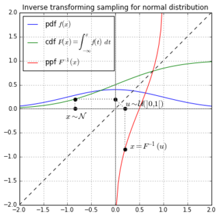
Inverse transform sampling is a basic method for pseudo-random number sampling, i.e., for generating sample numbers at random from any probability distribution given its cumulative distribution function.

<span class="mw-page-title-main">Exponential distribution</span> Probability distribution

In probability theory and statistics, the exponential distribution or negative exponential distribution is the probability distribution of the distance between events in a Poisson point process, i.e., a process in which events occur continuously and independently at a constant average rate; the distance parameter could be any meaningful mono-dimensional measure of the process, such as time between production errors, or length along a roll of fabric in the weaving manufacturing process. It is a particular case of the gamma distribution. It is the continuous analogue of the geometric distribution, and it has the key property of being memoryless. In addition to being used for the analysis of Poisson point processes it is found in various other contexts.

<span class="mw-page-title-main">Chi-squared distribution</span> Probability distribution and special case of gamma distribution

In probability theory and statistics, the chi-squared distribution with degrees of freedom is the distribution of a sum of the squares of independent standard normal random variables. The chi-squared distribution is a special case of the gamma distribution and is one of the most widely used probability distributions in inferential statistics, notably in hypothesis testing and in construction of confidence intervals. This distribution is sometimes called the central chi-squared distribution, a special case of the more general noncentral chi-squared distribution.

<span class="mw-page-title-main">Logit</span> Function in statistics

In statistics, the logit function is the quantile function associated with the standard logistic distribution. It has many uses in data analysis and machine learning, especially in data transformations.

<span class="mw-page-title-main">Weibull distribution</span> Continuous probability distribution

In probability theory and statistics, the Weibull distribution is a continuous probability distribution. It models a broad range of random variables, largely in the nature of a time to failure or time between events. Examples are maximum one-day rainfalls and the time a user spends on a web page.

<span class="mw-page-title-main">Gamma distribution</span> Probability distribution

In probability theory and statistics, the gamma distribution is a versatile two-parameter family of continuous probability distributions. The exponential distribution, Erlang distribution, and chi-squared distribution are special cases of the gamma distribution. There are two equivalent parameterizations in common use:

  1. With a shape parameter k and a scale parameter θ
  2. With a shape parameter and an inverse scale parameter , called a rate parameter.
<span class="mw-page-title-main">Logistic distribution</span> Continuous probability distribution

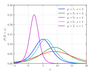
In probability theory and statistics, the logistic distribution is a continuous probability distribution. Its cumulative distribution function is the logistic function, which appears in logistic regression and feedforward neural networks. It resembles the normal distribution in shape but has heavier tails. The logistic distribution is a special case of the Tukey lambda distribution.

<span class="mw-page-title-main">Laplace distribution</span> Probability distribution

In probability theory and statistics, the Laplace distribution is a continuous probability distribution named after Pierre-Simon Laplace. It is also sometimes called the double exponential distribution, because it can be thought of as two exponential distributions spliced together along the abscissa, although the term is also sometimes used to refer to the Gumbel distribution. The difference between two independent identically distributed exponential random variables is governed by a Laplace distribution, as is a Brownian motion evaluated at an exponentially distributed random time. Increments of Laplace motion or a variance gamma process evaluated over the time scale also have a Laplace distribution.

Variational Bayesian methods are a family of techniques for approximating intractable integrals arising in Bayesian inference and machine learning. They are typically used in complex statistical models consisting of observed variables as well as unknown parameters and latent variables, with various sorts of relationships among the three types of random variables, as might be described by a graphical model. As typical in Bayesian inference, the parameters and latent variables are grouped together as "unobserved variables". Variational Bayesian methods are primarily used for two purposes:

  1. To provide an analytical approximation to the posterior probability of the unobserved variables, in order to do statistical inference over these variables.
  2. To derive a lower bound for the marginal likelihood of the observed data. This is typically used for performing model selection, the general idea being that a higher marginal likelihood for a given model indicates a better fit of the data by that model and hence a greater probability that the model in question was the one that generated the data.
<span class="mw-page-title-main">Pearson distribution</span> Family of continuous probability distributions

The Pearson distribution is a family of continuous probability distributions. It was first published by Karl Pearson in 1895 and subsequently extended by him in 1901 and 1916 in a series of articles on biostatistics.

<span class="mw-page-title-main">Empirical distribution function</span> Distribution function associated with the empirical measure of a sample

In statistics, an empirical distribution function is the distribution function associated with the empirical measure of a sample. This cumulative distribution function is a step function that jumps up by 1/n at each of the n data points. Its value at any specified value of the measured variable is the fraction of observations of the measured variable that are less than or equal to the specified value.

<span class="mw-page-title-main">Inverse Gaussian distribution</span> Family of continuous probability distributions

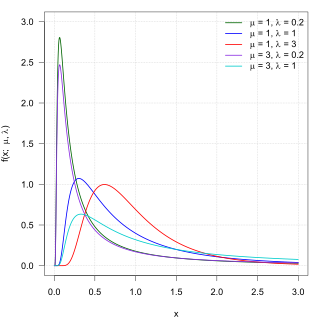
In probability theory, the inverse Gaussian distribution is a two-parameter family of continuous probability distributions with support on (0,∞).

Expected shortfall (ES) is a risk measure—a concept used in the field of financial risk measurement to evaluate the market risk or credit risk of a portfolio. The "expected shortfall at q% level" is the expected return on the portfolio in the worst of cases. ES is an alternative to value at risk that is more sensitive to the shape of the tail of the loss distribution.

In financial mathematics, tail value at risk (TVaR), also known as tail conditional expectation (TCE) or conditional tail expectation (CTE), is a risk measure associated with the more general value at risk. It quantifies the expected value of the loss given that an event outside a given probability level has occurred.

<span class="mw-page-title-main">Tukey lambda distribution</span>

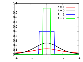
Formalized by John Tukey, the Tukey lambda distribution is a continuous, symmetric probability distribution defined in terms of its quantile function. It is typically used to identify an appropriate distribution and not used in statistical models directly.

<span class="mw-page-title-main">Conway–Maxwell–Poisson distribution</span> Probability distribution

In probability theory and statistics, the Conway–Maxwell–Poisson distribution is a discrete probability distribution named after Richard W. Conway, William L. Maxwell, and Siméon Denis Poisson that generalizes the Poisson distribution by adding a parameter to model overdispersion and underdispersion. It is a member of the exponential family, has the Poisson distribution and geometric distribution as special cases and the Bernoulli distribution as a limiting case.

<span class="mw-page-title-main">Poisson distribution</span> Discrete probability distribution

In probability theory and statistics, the Poisson distribution is a discrete probability distribution that expresses the probability of a given number of events occurring in a fixed interval of time if these events occur with a known constant mean rate and independently of the time since the last event. It can also be used for the number of events in other types of intervals than time, and in dimension greater than 1.

References

  1. Ehm, W.; Gneiting, T.; Jordan, A.; Krüger, F. (2016). "Of quantiles and expectiles: Consistent scoring functions, Choquet representations, and forecast rankings". J. R. Stat. Soc. B. 78 (3): 505–562. arXiv: 1503.08195 . doi: 10.1111/rssb.12154 .
  2. "Archived copy" (PDF). Archived from the original (PDF) on March 24, 2012. Retrieved March 25, 2012.{{cite web}}: CS1 maint: archived copy as title (link)
  3. Gilchrist, W. (2000). Statistical Modelling with Quantile Functions. ISBN   1-58488-174-7.
  4. Jaeckel, P. (2002). Monte Carlo methods in finance.
  5. Derflinger, Gerhard; Hörmann, Wolfgang; Leydold, Josef (2010). "Random variate generation by numerical inversion when only the density is known". ACM Transactions on Modeling and Computer Simulation. 20 (4). doi:10.1145/945511.945517.
  6. https://statmath.wu.ac.at/unuran/index.html
  7. https://cran.r-project.org/package=Runuran
  8. https://docs.scipy.org/doc/scipy/reference/stats.sampling.html
  9. Baumgarten, Christoph; Patel, Tirth (2022). "Automatic random variate generation in Python". Proceedings of the 21st Python in Science Conference. doi:10.25080/majora-212e5952-007.
  10. Steinbrecher, G., Shaw, W.T. (2008). "Quantile mechanics". European Journal of Applied Mathematics. 19 (2): 87–112. doi:10.1017/S0956792508007341. S2CID   6899308.{{cite journal}}: CS1 maint: multiple names: authors list (link)
  11. Wichura, M.J. (1988). "Algorithm AS241: The Percentage Points of the Normal Distribution". Applied Statistics. Blackwell Publishing. 37 (3): 477–484. doi:10.2307/2347330. JSTOR   2347330.
  12. An algorithm for computing the inverse normal cumulative distribution function Archived May 5, 2007, at the Wayback Machine
  13. Computational Finance: Differential Equations for Monte Carlo Recycling
  14. Shaw, W.T. (2006). "Sampling Student's T distribution – Use of the inverse cumulative distribution function". Journal of Computational Finance. 9 (4): 37–73. doi:10.21314/JCF.2006.150.
  15. Karvanen, J. (2006). "Estimation of quantile mixtures via L-moments and trimmed L-moments". Computational Statistics & Data Analysis. 51 (2): 947–956. doi:10.1016/j.csda.2005.09.014.

Further reading