Part of a series on statistics |
Probability theory |
---|
Given two random variables that are defined on the same probability space, [1] the joint probability distribution is the corresponding probability distribution on all possible pairs of outputs. The joint distribution can just as well be considered for any given number of random variables. The joint distribution encodes the marginal distributions, i.e. the distributions of each of the individual random variables and the conditional probability distributions, which deal with how the outputs of one random variable are distributed when given information on the outputs of the other random variable(s).
In the formal mathematical setup of measure theory, the joint distribution is given by the pushforward measure, by the map obtained by pairing together the given random variables, of the sample space's probability measure.
In the case of real-valued random variables, the joint distribution, as a particular multivariate distribution, may be expressed by a multivariate cumulative distribution function, or by a multivariate probability density function together with a multivariate probability mass function. In the special case of continuous random variables, it is sufficient to consider probability density functions, and in the case of discrete random variables, it is sufficient to consider probability mass functions.
Each of two urns contains twice as many red balls as blue balls, and no others, and one ball is randomly selected from each urn, with the two draws independent of each other. Let and be discrete random variables associated with the outcomes of the draw from the first urn and second urn respectively. The probability of drawing a red ball from either of the urns is 2/3, and the probability of drawing a blue ball is 1/3. The joint probability distribution is presented in the following table:
A=Red | A=Blue | P(B) | |
---|---|---|---|
B=Red | (2/3)(2/3)=4/9 | (1/3)(2/3)=2/9 | 4/9+2/9=2/3 |
B=Blue | (2/3)(1/3)=2/9 | (1/3)(1/3)=1/9 | 2/9+1/9=1/3 |
P(A) | 4/9+2/9=2/3 | 2/9+1/9=1/3 |
Each of the four inner cells shows the probability of a particular combination of results from the two draws; these probabilities are the joint distribution. In any one cell the probability of a particular combination occurring is (since the draws are independent) the product of the probability of the specified result for A and the probability of the specified result for B. The probabilities in these four cells sum to 1, as with all probability distributions.
Moreover, the final row and the final column give the marginal probability distribution for A and the marginal probability distribution for B respectively. For example, for A the first of these cells gives the sum of the probabilities for A being red, regardless of which possibility for B in the column above the cell occurs, as 2/3. Thus the marginal probability distribution for gives 's probabilities unconditional on , in a margin of the table.
Consider the flip of two fair coins; let and be discrete random variables associated with the outcomes of the first and second coin flips respectively. Each coin flip is a Bernoulli trial and has a Bernoulli distribution. If a coin displays "heads" then the associated random variable takes the value 1, and it takes the value 0 otherwise. The probability of each of these outcomes is 1/2, so the marginal (unconditional) density functions are
The joint probability mass function of and defines probabilities for each pair of outcomes. All possible outcomes are
Since each outcome is equally likely the joint probability mass function becomes
Since the coin flips are independent, the joint probability mass function is the product of the marginals:
Consider the roll of a fair die and let if the number is even (i.e. 2, 4, or 6) and otherwise. Furthermore, let if the number is prime (i.e. 2, 3, or 5) and otherwise.
1 | 2 | 3 | 4 | 5 | 6 | |
---|---|---|---|---|---|---|
A | 0 | 1 | 0 | 1 | 0 | 1 |
B | 0 | 1 | 1 | 0 | 1 | 0 |
Then, the joint distribution of and , expressed as a probability mass function, is
These probabilities necessarily sum to 1, since the probability of some combination of and occurring is 1.
If more than one random variable is defined in a random experiment, it is important to distinguish between the joint probability distribution of X and Y and the probability distribution of each variable individually. The individual probability distribution of a random variable is referred to as its marginal probability distribution. In general, the marginal probability distribution of X can be determined from the joint probability distribution of X and other random variables.
If the joint probability density function of random variable X and Y is , the marginal probability density function of X and Y, which defines the marginal distribution, is given by:
where the first integral is over all points in the range of (X,Y) for which X=x and the second integral is over all points in the range of (X,Y) for which Y=y. [2]
For a pair of random variables , the joint cumulative distribution function (CDF) is given by [3] : p. 89
(Eq.1) |
where the right-hand side represents the probability that the random variable takes on a value less than or equal to and that takes on a value less than or equal to .
For random variables , the joint CDF is given by
(Eq.2) |
Interpreting the random variables as a random vector yields a shorter notation:
The joint probability mass function of two discrete random variables is:
(Eq.3) |
or written in terms of conditional distributions
where is the probability of given that .
The generalization of the preceding two-variable case is the joint probability distribution of discrete random variables which is:
(Eq.4) |
or equivalently
This identity is known as the chain rule of probability.
Since these are probabilities, in the two-variable case
which generalizes for discrete random variables to
The joint probability density function for two continuous random variables is defined as the derivative of the joint cumulative distribution function (see Eq.1 ):
(Eq.5) |
This is equal to:
where and are the conditional distributions of given and of given respectively, and and are the marginal distributions for and respectively.
The definition extends naturally to more than two random variables:
(Eq.6) |
Again, since these are probability distributions, one has
respectively
The "mixed joint density" may be defined where one or more random variables are continuous and the other random variables are discrete. With one variable of each type
One example of a situation in which one may wish to find the cumulative distribution of one random variable which is continuous and another random variable which is discrete arises when one wishes to use a logistic regression in predicting the probability of a binary outcome Y conditional on the value of a continuously distributed outcome . One must use the "mixed" joint density when finding the cumulative distribution of this binary outcome because the input variables were initially defined in such a way that one could not collectively assign it either a probability density function or a probability mass function. Formally, is the probability density function of with respect to the product measure on the respective supports of and . Either of these two decompositions can then be used to recover the joint cumulative distribution function:
The definition generalizes to a mixture of arbitrary numbers of discrete and continuous random variables.
In general two random variables and are independent if and only if the joint cumulative distribution function satisfies
Two discrete random variables and are independent if and only if the joint probability mass function satisfies
for all and .
While the number of independent random events grows, the related joint probability value decreases rapidly to zero, according to a negative exponential law.
Similarly, two absolutely continuous random variables are independent if and only if
for all and . This means that acquiring any information about the value of one or more of the random variables leads to a conditional distribution of any other variable that is identical to its unconditional (marginal) distribution; thus no variable provides any information about any other variable.
If a subset of the variables is conditionally dependent given another subset of these variables, then the probability mass function of the joint distribution is . is equal to . Therefore, it can be efficiently represented by the lower-dimensional probability distributions and . Such conditional independence relations can be represented with a Bayesian network or copula functions.
When two or more random variables are defined on a probability space, it is useful to describe how they vary together; that is, it is useful to measure the relationship between the variables. A common measure of the relationship between two random variables is the covariance. Covariance is a measure of linear relationship between the random variables. If the relationship between the random variables is nonlinear, the covariance might not be sensitive to the relationship, which means, it does not relate the correlation between two variables.
The covariance between the random variables and is [4]
There is another measure of the relationship between two random variables that is often easier to interpret than the covariance.
The correlation just scales the covariance by the product of the standard deviation of each variable. Consequently, the correlation is a dimensionless quantity that can be used to compare the linear relationships between pairs of variables in different units. If the points in the joint probability distribution of X and Y that receive positive probability tend to fall along a line of positive (or negative) slope, ρXY is near +1 (or −1). If ρXY equals +1 or −1, it can be shown that the points in the joint probability distribution that receive positive probability fall exactly along a straight line. Two random variables with nonzero correlation are said to be correlated. Similar to covariance, the correlation is a measure of the linear relationship between random variables.
The correlation coefficient between the random variables and is
Named joint distributions that arise frequently in statistics include the multivariate normal distribution, the multivariate stable distribution, the multinomial distribution, the negative multinomial distribution, the multivariate hypergeometric distribution, and the elliptical distribution.
In probability theory and statistics, the cumulative distribution function (CDF) of a real-valued random variable , or just distribution function of , evaluated at , is the probability that will take a value less than or equal to .
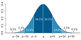
Independence is a fundamental notion in probability theory, as in statistics and the theory of stochastic processes. Two events are independent, statistically independent, or stochastically independent if, informally speaking, the occurrence of one does not affect the probability of occurrence of the other or, equivalently, does not affect the odds. Similarly, two random variables are independent if the realization of one does not affect the probability distribution of the other.
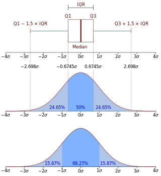
In probability theory, a probability density function (PDF), density function, or density of an absolutely continuous random variable, is a function whose value at any given sample in the sample space can be interpreted as providing a relative likelihood that the value of the random variable would be equal to that sample. Probability density is the probability per unit length, in other words, while the absolute likelihood for a continuous random variable to take on any particular value is 0, the value of the PDF at two different samples can be used to infer, in any particular draw of the random variable, how much more likely it is that the random variable would be close to one sample compared to the other sample.
In probability, and statistics, a multivariate random variable or random vector is a list or vector of mathematical variables each of whose value is unknown, either because the value has not yet occurred or because there is imperfect knowledge of its value. The individual variables in a random vector are grouped together because they are all part of a single mathematical system — often they represent different properties of an individual statistical unit. For example, while a given person has a specific age, height and weight, the representation of these features of an unspecified person from within a group would be a random vector. Normally each element of a random vector is a real number.
In probability theory and statistics, the multivariate normal distribution, multivariate Gaussian distribution, or joint normal distribution is a generalization of the one-dimensional (univariate) normal distribution to higher dimensions. One definition is that a random vector is said to be k-variate normally distributed if every linear combination of its k components has a univariate normal distribution. Its importance derives mainly from the multivariate central limit theorem. The multivariate normal distribution is often used to describe, at least approximately, any set of (possibly) correlated real-valued random variables, each of which clusters around a mean value.
In statistics, correlation or dependence is any statistical relationship, whether causal or not, between two random variables or bivariate data. Although in the broadest sense, "correlation" may indicate any type of association, in statistics it usually refers to the degree to which a pair of variables are linearly related. Familiar examples of dependent phenomena include the correlation between the height of parents and their offspring, and the correlation between the price of a good and the quantity the consumers are willing to purchase, as it is depicted in the so-called demand curve.
Covariance in probability theory and statistics is a measure of the joint variability of two random variables.
In probability theory and statistics, two real-valued random variables, , , are said to be uncorrelated if their covariance, , is zero. If two variables are uncorrelated, there is no linear relationship between them.
In probability theory and statistics, a covariance matrix is a square matrix giving the covariance between each pair of elements of a given random vector.
In probability theory and statistics, a Gaussian process is a stochastic process, such that every finite collection of those random variables has a multivariate normal distribution. The distribution of a Gaussian process is the joint distribution of all those random variables, and as such, it is a distribution over functions with a continuous domain, e.g. time or space.
In probability theory and information theory, the mutual information (MI) of two random variables is a measure of the mutual dependence between the two variables. More specifically, it quantifies the "amount of information" obtained about one random variable by observing the other random variable. The concept of mutual information is intimately linked to that of entropy of a random variable, a fundamental notion in information theory that quantifies the expected "amount of information" held in a random variable.
In probability theory and statistics, the marginal distribution of a subset of a collection of random variables is the probability distribution of the variables contained in the subset. It gives the probabilities of various values of the variables in the subset without reference to the values of the other variables. This contrasts with a conditional distribution, which gives the probabilities contingent upon the values of the other variables.
In probability and statistics, the Dirichlet distribution, often denoted , is a family of continuous multivariate probability distributions parameterized by a vector of positive reals. It is a multivariate generalization of the beta distribution, hence its alternative name of multivariate beta distribution (MBD). Dirichlet distributions are commonly used as prior distributions in Bayesian statistics, and in fact, the Dirichlet distribution is the conjugate prior of the categorical distribution and multinomial distribution.
In statistics and information theory, a maximum entropy probability distribution has entropy that is at least as great as that of all other members of a specified class of probability distributions. According to the principle of maximum entropy, if nothing is known about a distribution except that it belongs to a certain class, then the distribution with the largest entropy should be chosen as the least-informative default. The motivation is twofold: first, maximizing entropy minimizes the amount of prior information built into the distribution; second, many physical systems tend to move towards maximal entropy configurations over time.
This article discusses how information theory is related to measure theory.
In statistics, an exchangeable sequence of random variables is a sequence X1, X2, X3, ... whose joint probability distribution does not change when the positions in the sequence in which finitely many of them appear are altered. In other words, the joint distribution is invariant to finite permutation. Thus, for example the sequences
In probability theory, the family of complex normal distributions, denoted or , characterizes complex random variables whose real and imaginary parts are jointly normal. The complex normal family has three parameters: location parameter μ, covariance matrix , and the relation matrix . The standard complex normal is the univariate distribution with , , and .
In statistics and in probability theory, distance correlation or distance covariance is a measure of dependence between two paired random vectors of arbitrary, not necessarily equal, dimension. The population distance correlation coefficient is zero if and only if the random vectors are independent. Thus, distance correlation measures both linear and nonlinear association between two random variables or random vectors. This is in contrast to Pearson's correlation, which can only detect linear association between two random variables.
In probability theory and statistics, a complex random vector is typically a tuple of complex-valued random variables, and generally is a random variable taking values in a vector space over the field of complex numbers. If are complex-valued random variables, then the n-tuple is a complex random vector. Complex random variables can always be considered as pairs of real random vectors: their real and imaginary parts.
Poisson-type random measures are a family of three random counting measures which are closed under restriction to a subspace, i.e. closed under thinning. They are the only distributions in the canonical non-negative power series family of distributions to possess this property and include the Poisson distribution, negative binomial distribution, and binomial distribution. The PT family of distributions is also known as the Katz family of distributions, the Panjer or (a,b,0) class of distributions and may be retrieved through the Conway–Maxwell–Poisson distribution.
{{cite book}}
: CS1 maint: location missing publisher (link){{cite book}}
: CS1 maint: location missing publisher (link)